Distributed Unsupervised Deep Learning: Real-Time Financial Fraud detection using AI Pipeline for Spark Structured Streaming, BigDL & Analytics Zoo with Apache Kafka on Hadoop cluster

Distributed Processing, Apache Spark, Spark DataFrame , Spark RDD, ML Pipeline, Task scheduling, BigDL, Analytic zoo, Model quantisation, Distributed training, Hadoop HDFS, Hadoop YARN, Grafana Dashboard, Prometheus, Grafana Loki, Supervised Learning, Semi Supervised Learning, Unsupervised Learning, Reinforcement Learning, Auto encoder, Convolution Neural Networks(CNN) Auto encoder, Variational Auto-encoders, Adversarial auto-encoders, Generative adversarial network (GAN), Autoencoder GANs, Transfer Learning, Deep Embedded Clustering with Autoencoder, Deep Clustering, Deep Embedded Clustering with GAN, Deep Embedded Clustering with CNN
In this article, I will explain all concepts of Distributed Deep Learning-based fraud detection by using Apache Spark structured streaming and Apache Kafka on the Hadoop cluster. We will also implement this concept and visualize the results on the Dashboard with help of Grafana, Prometheus, and Loki.
1. INTRODUCTION
A. Distributed Computing
A distributed system or distributed computing is a system with multiple components located on different machines that communicate and coordinate actions in order to appear as a single coherent system to the end-user.
The distributed machines may be computers, physical servers, virtual machines, containers, or any other node that can connect to the network, have local memory, and communicate by passing messages.
The functions of distributed systems are,1. In this, Each machine work towards a common goal and the end-user view results as one cohesive unit.2.Each machine has its own end-user and the distributed system facilitates sharing resources or communication services.
The distributed system have usually three primary features:
a. All components run concurrently
b. There is no global clock
c. All components fail independently of each other.
The Distributed systems have endless use cases, a few being electronic banking systems, massively multiplayer online games, and wireless sensor networks.
Distributed systems Benefits and challenges
For the implementation of Distributed system, there are mainly three reasons that decision to be taken for implementation of this concept:
i. Horizontal Scalability — Computing happens independently on each node. it is inexpensive and very easy to add additional nodes and functionality if required.ii. Reliability — Most distributed systems are fault-tolerant as they can be made up of hundreds of nodes that work together. Incase of any single machine failure, System generally doesn’t experience any disruptions.iii. Performance — Distributed systems are extremely efficient because workloads can be broken up and sent to multiple machines.
So we can say that the complex architectural design, construction, and debugging processes that are required to create an effective distributed system can be more powerful.
Types of distributed systems:
The Distributed system mainly have four different basic architecture models:
i. Client-server Type: Clients contact the server for data, then format it and display it to the end-user. The end-user can also make a change from the client-side and commit it back to the server to make it permanent.ii. Three-tier: Information about the client is stored in a middle-tier rather than on the client to simplify application deployment. This architecture model is most common for web applications.iii. N-tier: Generally used when an application or server needs to forward requests to additional enterprise services on the network.iv. Peer-to-peer: In this, There are no additional machines used to provide services or manage resources. Responsibilities are uniformly distributed among machines in the system, known as peers, which can serve as either client or server.
Comparison between Parallel and Distributed computing
Parallel computing consists of multiple processors that communicate with each other using shared memory, but in the case of Distributed computing, multiple processors connected by a communication network where the messages are sent over the network.

Now based on Github and Stack Overflow activity, as well as Google Search results. In the figure below is a ranking of the top 20 of 140 distributed computing packages that are useful for Data Science.

The above table shows standardized scores, where a value of 1 means one standard deviation above average (average = score of 0). For example, Apache Hadoop is 6.6 standard deviations above average in Stack Overflow activity, while Apache Flink is close to average. See below for methods.
B. Apache Spark
Apache Spark is a general-purpose fast clustering computing open-source framework that is used as a wide range of data processing engines. Apache Spark reveals development API’s, which also qualify data workers to accomplish streaming, machine learning, or SQL workloads that demand repeated access to data sets. It can perform batch processing and stream processing where Stream processing means dealing with Spark streaming data and Batch processing refers to the processing of the previously collected job in a single batch. It can integrate with all the Big data tools. Like spark can access any Hadoop data source, also can run on Hadoop clusters. Furthermore, Apache Spark extends Hadoop MapReduce to the next level. That also includes iterative queries and stream processing. Basically, Spark is independent of Hadoop since it has its own cluster management system, it uses Hadoop for storage purposes only.
Advantages of Apache Spark
i. Dynamic in Nature: In Memory cluster computation capability.ii. Speed: Increases the processing speed of an application. spark is 100x faster than mapreduce.iii. Ease of Use & Advanced Analyticsiv. Multilingual: Supports many languages such as Scala, R, Python, JAVAvi. Open Source & Increasing Access to Big Datavii. Low-level transformation and actions and control on your dataset.viii. Data is unstructured, such as media streams or streams of text.ix. We can manipulate data with functional programming constructs than domain-specific expressions.
Apache Spark Architecture Pipeline
A Java virtual machine (JVM) is a cross-platform runtime engine that can execute instructions compiled into Java bytecode. Scala, which Spark is written in, compiles into bytecode and runs on JVMs. In JVM all Spark components, including the Driver, Master, and Executor processes run.
In the Spark program, each component has a specific role. Some of these roles, such as the client components, are passive during execution; other roles are active in the execution of the program, including components executing computation functions. The components of a Spark application are i. driver ii. Master iii. Cluster manager iv. Executors
The Architecture of Apache Spark is shown below,

In Apache Spark, Resilient Distributed Datasets (RDD) are used to store data. Spark RDD is an immutable collection of objects & it divides data into logical partitions. Because of this logical partition, it can process each part in parallel, in different nodes of the cluster. We can enhance the computation process of Spark by caching RDD. Task parallelism and in-memory computing are the keys to being ultra-fast.
The steps shown below Figure are:
i. The client submits a Spark application to the cluster manager (the YARN ResourceManager). The driver process, SparkSession, and SparkContext are created and run on the client.ii. The ResourceManager assigns an ApplicationMaster (the Spark master) for the application.iii. The ApplicationMaster requests containers to be used for executors from the ResourceManager. With the containers assigned, the executors spawn.iv. The driver, located on the client, then communicates with the executors to marshal processing of tasks and stages of the Spark program. The driver returns the progress, results, and status to the client.
The client deployment mode is the simplest mode to use. However, it lacks the resiliency required for most production applications.

Internal Job Execution on Apache Spark
Spark translates the RDD transformations into something called DAG (Directed Acyclic Graph) and starts the execution. At the high level, when any action is called on the RDD, Spark creates the DAG and submits it to the DAG scheduler.
i. The DAG scheduler divides operators into stages of tasks. A stage is comprised of tasks based on partitions of the input data. The DAG scheduler pipelines operators together. For e.g. Many map operators can be scheduled in a single stage. The final result of a DAG scheduler is a set of stages.ii. The Stages are passed on to the Task Scheduler. The task scheduler launches tasks via cluster manager.(Spark Standalone/Yarn/Mesos). The task scheduler doesn’t know about dependencies of the stages.iii. The Worker executes the tasks on the Slave.
The below figure shows how internal job execution can happen on Spark,

More details about the DAG scheduler we will discuss later.
Resilient Distributed Datasets (RDD)
RDD is the core of spark as its distributed among various nodes of the cluster that leverages data locality. An RDD is a collection of immutable datasets is partitioned into one or many partitions. To achieve parallelism inside the application, Partitions are the units for it. Repartition or coalesce transformations can help to maintain the number of partitions. Data access is optimized utilizing RDD shuffling. As Spark is close to data, it sends data across various nodes through it and creates required partitions as needed.
Decomposing the name RDD:
i. Resilient, i.e. fault-tolerant with the help of RDD lineage graph (DAG) and so able to recomputed the missing or damaged partitions due to node failures.ii. Distributed, since Data resides on multiple nodes.iii. Dataset represents records of the data you work with. The user can load the data set externally which can be either JSON file, CSV file, text file or database via JDBC with no specific data structure.
History of Apache Spark APIs:

The key motivations behind the concept of RDD are-
i. Iterative algorithms.ii. Interactive data mining tools.iii. Distributed Shared Memory (DSM) is a very general abstraction, but this generality makes it harder to implement in an efficient and fault-tolerant manner on commodity clusters.iv. In distributed computing system data is stored in an intermediate stable distributed store such as HDFS or Amazon S3. v. In-memory Computationvi. Lazy Evaluations: Spark computes transformations when an action requires a result for the driver program.vii. Persistence,viii. Coarse grained operations: It applies to all elements in datasets through maps or filter or group by operation.
In the first two cases we keep data in-memory, it can improve performance by an order of magnitude. The main challenge in designing RDD is defining a program interface that provides fault tolerance efficiently. To achieve fault tolerance efficiently, RDDs provide a restricted form of shared memory, based on coarse-grained transformation rather than fine-grained updates to shared state.
Spark RDD Operations
There are basically two types of operations Apache Spark RDD can perform,
i. Transformations:
Transformations are lazy operations on an RDD in Apache Spark. It creates one or many new RDDs, which executes when an Action occurs. Spark RDD Transformations are functions that take an RDD as the input and produce one or many RDDs as the output. They do not change the input RDD, but always produce one or more new RDDs by applying the computations they represent. The basic RDD Transformations operations are: Map(), filter(), reduceByKey(), mapPartitions(), mapPartitionsWithIndex(), groupBy(), sortByetc(). Certain transformations can be pipelined which is an optimization method, that Spark uses to improve the performance of computations. There are two kinds of transformations: narrow transformation, wide transformation.
There are two types of Transformations, Narrow Transformation (Map, FlatMap, Filter, Sample, Union, MapPartition) and Wide Transformations (Intersection, ReduceByKey, Distinct, GroupByKey, Join, Cartesian, Repartition, Coalesce)

ii. Actions:
An Action in Spark returns the final result of RDD computations. It triggers execution using lineage graph ( Lineage graph is dependency graph of all parallel RDDs of RDD) to load the data into original RDD, carry out all intermediate transformations and return final results to Driver program or write it out to file system. Actions are RDD operations that produce non-RDD values. They materialize a value in a Spark program. An Action is one of the ways to send results from executors to the driver. Some of action methods in Apache Spark are: First(), take(), reduce(), collect(), the count().
Note:
Using transformations, one can create RDD from the existing one. But when we want to work with the actual dataset, at that point we use Action. When the Action occurs it does not create the new RDD, unlike transformation. Thus, actions are RDD operations that give no RDD values. Action stores its value either to drivers or to the external storage system. It brings the laziness of RDD into motion.
Spark Driver (Master Process)
Apache Spark Driver is the process that clients use to submit applications in the Spark program. The Driver is responsible for planning and coordinating the execution of the Spark program and returning status and/or results (data) to the client and It is also responsible for creating the Spark Session. The Driver can physically reside on a client or on a node in the cluster.
The Spark Driver converts the programs into tasks and schedules the tasks for Executors. The Task Scheduler is the part of the Driver and helps to distribute tasks to Executors. The Spark Session object represents a connection to a Spark cluster. The Spark Session is instantiated at the beginning of a Spark application, including the interactive shells, and is used for the entirety of the program.
The driver prepares the context and declares the operations on the data using RDD transformations and actions.
i. The driver submits the serialized RDD graph to the master. The master creates tasks out of it and submits them to the workers for execution. It coordinates the different job stages.ii. The workers is where the tasks are actually executed. They should have the resources and network connectivity required to execute the operations requested on the RDDs.
In below figure shows that how Spark Driver work with TaskScheduler for a single SparkContext,

Spark Cluster Manager
In Apache Spark, Cluster Manager is the core part that allows is to launch of executors sometimes drivers can be launched by it also. Spark Scheduler schedules the actions and jobs in Spark Application in FIFO way on cluster manager itself.
A good example of the Cluster Manager function is the YARN ResourceManager process for Spark applications running on Hadoop clusters. The ResourceManager schedules allocate and monitor the containers running on YARN NodeManagers. Spark applications then use these containers to host Executor processes, as well as the Master process if the application is running in cluster mode. The below figure shows that YARN Resource Manager and Node Manager framework architecture,

Cluster Manager keeps track of the available resources (nodes) available in the cluster. When the SparkContext object is created, it connects to the cluster manager to negotiate for executors. From the available nodes, the cluster manager allocates some or all of the executors to the SparkContext based on the demand. Specifically, to run on a cluster, SparkContext can connect to several types of Cluster Managers, which allocate resources across applications. Once the connection is established, Spark acquires executors on the nodes in the cluster to run its processes, does some computations, and stores data for your application. Next, it sends your application code (defined by JAR or Python files passed to SparkContext) to the executors. Finally, SparkContext sends tasks to the executors to run. The below figure shows how ResourceManager, NodeManager, Application Master, and Containers work together.

Types of cluster managers
i. Standalone
In the Standalone cluster manager process, The execution mode uses Resource Manager for a spark job. Moreover, Spark allows us to create distributed master-slave architecture, by configuring properties file under $SPARK_HOME/conf directory. By default, it is set as a single node cluster just like Hadoop's pseudo-distribution mode. The Spark standalone mode requires each application to run an executor on every node in the cluster. Spark distribution comes with its own resource manager also. It has masters and a number of workers with the configured amount of memory and CPU cores. In Spark standalone cluster mode, Spark allocates resources based on the core. By default, an application will grab all the cores in the cluster.
Standalone is good for small Spark clusters, but it is not good for bigger clusters. Standalone is not recommended for bigger production clusters, because there is an overhead of running Spark daemons master-slave in cluster nodes. These daemons require dedicated resources.
A Spark standalone cluster with an application in cluster-deploy mode. A master and one worker are running on node 1, and the second worker is running on node 2. Workers are spawning drivers’ and executors’ JVMs.

To view cluster and job statistics it has a Web UI. It also has detailed log output for each job. The Spark Web UI will reconstruct the application’s UI after the application exists if an application has logged events for its lifetime.
ii. YARN Cluster Managers
In YARN, we can configure the number of executors for the Spark application. Here in each application instance has an ApplicationMaster process, which is the first container started for that application. The application is responsible for requesting resources from the ResourceManager, and, when allocated them, instructing NodeManagers to start containers on its behalf. ApplicationMasters eliminate the need for an active client and the process starting the application can terminate, and coordination continues from a process managed by YARN running on the cluster. Apache Spark with YARN can be deployed in two different modes,
i. Cluster Deployment Mode
In this mode, SparkDriver runs in the Application Master on Cluster host. A single process in a YARN container is responsible for both driving the application and requesting resources from YARN. The client that launches the application does not need to run for the lifetime of the application. Cluster mode is not well-suited for using Spark interactively. Spark applications that require user input, such as spark-shell and pyspark, require the Spark driver to run inside the client process that initiates the Spark application.

ii. Client Deployment Mode
In client mode, the Spark driver runs on the host where the job is submitted. The Application Master is responsible only for requesting executor containers from YARN. After the containers start, the client communicates with the containers to schedule work. It supports spark-shell, as the driver runs at the client-side.

Hadoop YARN has a Web UI for the ResourceManager and the NodeManager. The ResourceManager UI provides metrics for the cluster and the NodeManager provides information for each node, the applications, and containers running on the node.
iii. Mesos
Mesos framework consists of a master daemon that manages the agent daemons that are running on each cluster node. The master enables fine-grained sharing of resources (CPU, RAM) across frameworks by giving them resource offers. The master decides how many resources to offer to each framework according to a given organizational policy, such as fair sharing or strict priority.

A framework running on top of Mesos consists of two components:
i. A scheduler that registers with the master to be offered resources.ii. An executor process that is launched on agent nodes to run the framework’s tasks.
Mesos handles the workload in a distributed environment by dynamic resource sharing and isolation. It is helpful for the deployment and management of applications in large-scale cluster environments.
The three components of Apache Mesos are Mesos masters, Mesos slave, Frameworks.
i. Mesos Master is an instance of the cluster. A cluster has many Mesos masters that provide fault tolerance. Here one instance is the leading master.ii. Mesos Slave is a Mesos instance that offers resources to the cluster.iii. Mesos Master assigns the task to the slave. Mesos Framework allows applications to request the resources from the cluster. Thus, the application can perform the task.
It supports per container network monitoring and isolation. It provides many metrics for master and slave nodes accessible with URL. These metrics include percentage and number of allocated CPU’s, memory usage, etc.
Apache Spark Executors (Slave Processes)
An Apache Spark executor is a process launched for an application on a worker node, that runs tasks and keeps data in memory or disk storage across them. Each application has its own executors. Executors will always run till the lifecycle of a spark application once they are launched. Failed executors don’t stop the execution of spark job. Executor resides in the Worker node. Executors are launched at the start of a Spark Application in coordination with the Cluster Manager. They are dynamically launched and removed by the Driver as required.
The Responsibility of Apache Spark executor are:
i. To run an individual Task and return the result to the Driver.ii. It can cache (persist) the data in the Worker node.
We can have as many executors in Spark as data nodes. Moreover also possible to have as many cores as you can get from the cluster. The other way to describe Apache Spark Executor is either by their id, hostname, environment (as SparkEnv), or classpath. The most important point to note is Executor backends exclusively manage Executor in Spark. The following diagram depicts the architecture of TensorFlowOnSpark (TFoS).

The following pictures show Spark’s executor memory compartments when running:

For more detail about spark executor memory compartments when running you can read Apache Spark and memory.
Directed Acyclic Graph (DAG)
DAG is a graph that holds the track of operations applied on RDD. Spark tends to generate an operator graph when we enter our code to the Spark console. When an action is triggered to Spark RDD, Spark submits that graph to the DAGScheduler. It then divides those operator graphs into stages of the task inside the DAGScheduler. Every step may contain jobs based on several partitions of the incoming data. For Instance, Map operator graphs schedule for a single stage, and these stages pass on to the Task Scheduler in the cluster manager for their execution. This is the task of Work or Executors to execute these tasks on the slave.
Concepts of Apache Spark DAG,
i. Directed — Means which is directly connected from one node to another. This creates a sequence i.e. each node is in linkage from earlier to later in the appropriate sequence.ii. Acyclic — Defines that there is no cycle or loop available. Once a transformation takes place it cannot returns to its earlier position.iii. Graph — From graph theory, it is a combination of vertices and edges. Those pattern of connections together in a sequence is the graph.
The below figure shows that Working of DAGScheduler,

Apache Spark Lineage Graph
In Spark, Lineage Graph is a dependencies graph in between existing RDD and new RDD or if we want to recover the lost data from the lost persisted RDD. It means that all the dependencies between the RDD will be recorded in a graph, rather than the original data.
In the below figure, The Lineage graph of joining inputs from Input 1 with Input2. After reading from Input 1, Spark filters the read values to get only required values. Values from both inputs are combined and stored as an output.

Difference between Lineage Graph vs DAG Schedular:
i. Lineage Graph is dealing with only RDDs so it is applicable to transformations.ii. DAG(Directed Acyclic Graph) dealing with both transformation and actionsiii. DAG allows the user to dive into the stage and expanded details on any stage.
Apache Spark Ecosystem
Apache Spark is the leading platform for large-scale SQL, batch processing, stream processing, and machine learning, with an easy-to-use API. Apache Spark supports many different programming languages like Java, Scala, Python, R, and SQL.

In the figure above, We can see that the Spark ecosystem covers components such as Spark core component, Spark SQL, Spark Streaming, Spark MLlib, Spark GraphX, BigDL, and SparkR.
Apache Spark DataFrame
A DataFrame is conceptually equivalent to a table in a relational database. It is a dataset that is organized into named columns. The DataFrames can be constructed from a wide array of sources such as structured data files, tables in Hive, external databases, or existing RDDs. The DataFrame API is available in Scala, Java, Python, and R. In Scala and Java, a DataFrame is represented by a Dataset of Rows. In the Scala API, DataFrame is simply a type alias of Dataset[Row]. While, in Java API, users need to use Dataset<Row> to represent a DataFrame.
Features of DataFrame in Apache Spark,
i. Ability to process the data in the size of Kilobytes to Petabytes on a single node cluster to a large cluster.ii. Supports different data formats (Avro, csv, elastic search, and Cassandra) and storage systems (HDFS, HIVE tables, mysql, etc).iii. State of art optimization and code generation through the Spark SQL Catalyst optimizer (tree transformation framework).iv. Can be easily integrated with all Big Data tools and frameworks via Spark-Core.v. Provides API for Python, Java, Scala, and R Programming.
Comparison between DataFrames vs RDDs vs Datasets,

Apache Spark SQL
Apache Spark SQL brings native support for SQL to Spark and streamlines the process of querying data stored both in RDDs and in external sources. Spark SQL conveniently blurs the lines between RDDs and relational tables. It is used for structured data processing. It provides a programming abstraction called DataFrames and can also act as a distributed SQL query engine. It enables unmodified Hadoop Hive queries to run up to 100x faster on existing deployments and data. It also provides powerful integration with the rest of the Spark ecosystem (e.g., integrating SQL query processing with machine learning).
Apache Spark SQL makes it easy for developers to intermix SQL commands querying external data with complex analytics, all within a single application. Concretely, Spark SQL will allow developers to:
i. Import relational data from Parquet files and Hive tablesii. Run SQL queries over imported data and existing RDDsiii. Easily write RDDs out to Hive tables or Parquet filesiv. Using SQL we can query data, both from inside a Spark program and from external tools. The external tool connects through standard database connectors (JDBC/ODBC) to Spark SQL.v. The data can be read and written in a variety of structured formats. For example, JSON, Hive Tables, and Parquet.
Apache Spark SQL also includes a cost-based optimizer, columnar storage, and code generation to make queries fast. At the same time, it scales to thousands of nodes and multi-hour queries using the Spark engine, which provides full mid-query fault tolerance, without having to worry about using a different engine for historical data.
The Spark SQL supports only a subset of SQL functionality and users have to write code in Java, Python, and so on to execute a query. The advantages of Apache Spark SQL,

The architecture of Apache Spark SQL & HIVE is shown below,

Apache Spark SQL is faster than Hive when it comes to processing speed. Below The Limitations with Hive are:
i. Hive launches MapReduce jobs internally for executing the ad-hoc queries. MapReduce lags in the performance when it comes to the analysis of medium-sized datasets (10 to 200 GB).ii. Hive has no resume capability. This means that if the processing dies in the middle of a workflow, you cannot resume from where it got stuck.iii. Hive cannot drop encrypted databases in cascade when the trash is enabled and leads to an execution error. To overcome this, users have to use the Purge option to skip trash instead of drop.
Difference between Apache HIVE and Apache Spark SQL,

For more details, you can read: https://www.educba.com/apache-hive-vs-apache-spark-sql/
Apache Spark Streaming
For the processing of data streams, Apache Spark Streaming is an extension of the core Spark API. It provides a high-level abstraction called discretized stream or DStream, which represents a continuous stream of data. Internally, a DStream is represented as a sequence of RDDs. Spark streaming can receive input data streams from sources such as Kafka, Twitter, or TCP sockets. It then divides the data into batches, which are then processed by the Spark engine to generate the final stream of results in batches. Finally, the results can be pushed out to file systems, databases, or live dashboards. The Spark Streaming to seamlessly integrate with any other Spark components like MLlib and Spark SQL. Spark Streaming is different from other systems that either has a processing engine designed only for streaming or have similar batch and streaming APIs but compile internally to different engines. Spark’s single execution engine and unified programming model for batch and streaming lead to some unique benefits over other traditional streaming systems.
Spark Streaming has the following advantages,
i. Fast recovery from failures and stragglersii. Better load balancing and resource usageiii. Combining of streaming data with static datasets and interactive queriesiv. Native integration with advanced processing libraries (SQL, machine learning, graph processing)
A query on the input generates a result table. At every trigger interval (say, every 1 second), new rows are appended to the input table, which eventually updates the result table. Whenever the result table is updated, the changed result rows are written to an external sink. The output is defined as what gets written to external storage. The output can be configured in different modes:
i. Complete Mode: The entire updated result table is written to external storage. It is up to the storage connector to decide how to handle the writing of the entire table.ii. Append Mode: Only new rows appended in the result table since the last trigger are written to external storage. This is applicable only for the queries where existing rows in the Result Table are not expected to change.iii. Update Mode: Only the rows that were updated in the result table since the last trigger are written to external storage. This is different from Complete Mode in that Update Mode outputs only the rows that have changed since the last trigger. If the query doesn’t contain aggregations, it is equivalent to Append mode.

Sensors, IoT devices, social networks, and online transactions all generate data that needs to be monitored constantly and acted upon quickly. This unification of disparate data processing capabilities is the key reason behind Spark Streaming’s rapid adoption. It makes it very easy for developers to use a single framework to satisfy all their processing needs.

Apache Spark Machine Learning Pipeline
MLlib Package
MLlib is Spark’s machine learning (ML) library. Its goal is to make practical machine learning scalable and easy. At a high level, it provides tools such as:
i. ML Algorithms: common learning algorithms such as classification, regression, clustering, and collaborative filteringii. Featurization: feature extraction, transformation, dimensionality reduction, and selectioniii. Pipelines: tools for constructing, evaluating, and tuning ML Pipelinesiv. Persistence: saving and load algorithms, models, and Pipelinesv. Utilities: linear algebra, statistics, data handling, etc.
Spark.ml is a new package introduced in Spark 1.2, which aims to provide a uniform set of high-level APIs that help users create and tune practical machine learning pipelines. Spark ML standardizes APIs for machine learning algorithms to make it easier to combine multiple algorithms into a single pipeline, or workflow.
The list of Spark ML API are,
i. ML Dataset: Spark ML uses the SchemaRDD from Spark SQL as a dataset which can hold a variety of data types. E.g., a dataset could have different columns storing text, feature vectors, true labels, and predictions.ii. Transformer: A Transformer is an algorithm which can transform one SchemaRDD into another SchemaRDD by implementing transform() method. E.g., an ML model is a Transformer which transforms an RDD with features into an RDD with predictions. A Transformer is an abstraction for feature transformer and learned model. It converts one DataFrame to another DataFrame. It appends one or more columns to a DataFrame. In a feature transformer a DataFrame is the input and the output is a new DataFrame with a new mapped column.iii. Estimator: An Estimator is an algorithm which can be fit on a SchemaRDD to produce a Transformer. E.g., a learning algorithm is an Estimator which trains on a dataset and produces a model.iv. Pipeline: A Pipeline chains multiple Transformers and Estimators together to specify an ML workflow. The ML Pipelines is a High-Level API for MLlib that lives under the “spark.ml” package. A pipeline consists of a sequence of stages. There are two basic types of pipeline stages: Transformer and Estimator.v. Param: All Transformers and Estimators now share a common API for specifying parameters.
A big benefit of using ML Pipelines is hyperparameter optimization. The pipeline structure of Apache Spark is shown below,

Apache Spark GraphX
The Apache Spark GraphX is the Spark API for graphs and graph-parallel computation. It includes a growing collection of graph algorithms and builders to simplify graph analytics tasks.

At a high level, GraphX extends the Spark RDD by introducing a new Graph abstraction: a directed multigraph with properties attached to each vertex and edge.
Suppose we want to construct a property graph consisting of the various collaborators on the GraphX project. The vertex property might contain the username and occupation. GraphX supports property multigraph, which is a directed graph with multiple parallel edges to represent more than one relationship between the same source node & destination node. We could annotate edges with a string describing the relationships between collaborators:

The Apache GraphX extends the Spark RDD with a Resilient Distributed Property Graph. The property graph is a directed multigraph that can have multiple edges in parallel. Every edge and vertex have user-defined properties associated with it. The parallel edges allow multiple relationships between the same vertices. The GraphX library provides graph operators like subgraph, join Vertices, and aggregate Messages to transform the graph data. It provides several ways of building a graph from a collection of vertices and edges in an RDD or on a disk. GraphX also includes a number of graph algorithms and builders to perform graph analytics tasks. The Apache GraphX is different from other graph-processing frameworks in that it can perform both graph analytics and ETL and can do graph analysis on data that is not in graph form. Spark Graphx provides an implementation of various graph algorithms such as PageRank, Connected Components, and Triangle Counting.
Property graphs are immutable just like RDD, which means once we create the graph it cannot be modified but, we can transform it to create new graphs.
i. Property graphs distributed on multiple machines (executors) for parallel processing.ii. Property graphs are fault-tolerant, which means it can recreate in case of any failures.iii. In Spark GraphX, nodes and relationships are represented as dataframes or RDDS. Node dataframe must have a unique id along with other properties and the relationship dataframe must have a source and destination id along with other attributes.
Apache Spark Big DL
BigDL is a distributed deep learning framework built for a Big Data platform using Apache Spark. It combines the benefits of “high-performance computing” and “Big Data” architecture, providing native support for deep learning functionalities in Spark. Using BigDL, you can write deep learning applications as Scala or Python* programs and take advantage of the power of scalable Spark clusters. BigDL has evolved into a vibrant open-source project since Intel introduced it in December of 2016.
BigDL allows deep learning applications to run on the Apache Hadoop/Spark cluster so as to directly process the production data, and as a part of the end-to-end data analysis pipeline for deployment and management. The “model forward-backward” spark job, which computes the local gradients for each model replica in parallel.

You may want to use BigDL to write your deep learning programs if:
i. You want to analyze a large amount of data on the same big data Spark cluster on which the data reside (in, say, HDFS, Apache HBase*, or Hive);ii. You want to add deep learning functionality (either training or prediction) to your big data (Spark) programs or workflowiii. You want to use existing Hadoop/Spark clusters to run your deep learning applications, which you can then easily share with other workloads (e.g., extract-transform-load, data warehouse, feature engineering, classical machine learning, graph analytics).
To make it easy to build Spark and BigDL applications, a high-level Analytics Zoo is provided for end-to-end analytics + AI pipelines.
i. Rich deep learning support. Modeled after Torch, BigDL provides comprehensive support for deep learning, including numeric computing (via Tensor) and high level neural networks; in addition, users can load pre-trained Caffe or Torch models into Spark programs using BigDL.ii. Extremely high performance. To achieve high performance, BigDL uses Intel MKL / Intel MKL-DNN and multi-threaded programming in each Spark task. Consequently, it is orders of magnitude faster than out-of-box open source Caffe, Torch or TensorFlow on a single-node Xeon (i.e., comparable with mainstream GPU). With adoption of Intel DL Boost, BigDL improves inference latency and throughput significantly.iii. Efficiently scale-out. BigDL can efficiently scale out to perform data analytics at “Big Data scale”, by leveraging Apache Spark (a lightning fast distributed data processing framework), as well as efficient implementations of synchronous SGD and all-reduce communications on Spark.
BigDL Integration with Spark Streaming,

The BigDL library supports Spark versions 1.5, 1.6, and 2.0 and allows for deep learning to be embedded in existing Spark-based programs. It contains methods to convert Spark RDDs to a BigDL DataSet and can be used directly with Spark ML Pipelines.
BigDL Run as standard Apache Spark Program,

In Parameter synchronization in BigDL, each local gradient is evenly divided into N partitions; then each task n in the “parameter synchronization” job aggregates these local gradients and updates the weights for the nth partition.
Parameter Synchronization in BigDL,

Some end-to-end workflow of real-time streaming on Kafka, Spark Streaming, and BigDL,
Speech Recognition using BigDL,

InApache Spark pipeline first reads hundreds of millions of pictures from a distributed database into Spark (as an RDD of pictures) and then pre-processes the RDD of pictures in a distributed fashion using Spark. It then uses BigDL to load an SSD model (pre-trained in Caffe) for large-scale, distributed object detection on Spark, which generates the coordinates and scores for the detected objects in each of the pictures.
Here is the End-to-end object detection and image feature extraction pipeline (using SSD and DeepBit models) on top of Spark and BigDL.

Highlights of the BigDL v0.3.0 release
Since its initial open-source release in December 2016, BigDL has been used to build applications for fraud detection, recommender systems, image recognition, and many other purposes. The recent BigDL v0.3.0 release addresses many user requests, improving usability and add new features and functionality:
• New layers support• RNN encoder-decoder (sequence-to-sequence) architecture• Variational auto-encoder• 3D de-convolution• 1D convolution and pooling• Model quantization support• Quantize existing (BigDL, Caffe, Torch or TensorFlow) model• Converting float points to integer for model inference (for model size reduction & inference speedup)• Sparse tensor and layers — Efficient support of sparse data
For more detail, about BigDL you can read https://medium.com/@gdfilla/using-bigdl-in-data-science-experience-for-deep-learning-on-spark-f1cf30ad6ca0
Apache Spark Analytic Zoo
Apache Analytics Zoo seamlessly scales TensorFlow, Keras and PyTorch to distributed big data (using Spark, Flink & Ray). Analytics Zoo provides unified analytics & AI platform that seamlessly unites Spark, TensorFlow, Keras, and BigDL programs into an integrated data pipeline.
The entire data pipeline can then transparently scale out to a large Hadoop/Spark cluster for distributed training or inference.
i. Data wrangling and analysis using PySparkii. Deep learning model development using TensorFlow or Kerasiii. Distributed training/inference on Spark and BigDLiv. All within a single unified pipeline and in a user-transparent fashion!
In addition, Analytics Zoo also provides a rich set of analytics and AI support for the end-to-end pipeline, including
i. Easy-to-use abstractions and APIs (e.g., transfer learning support, autograd operations, Spark DataFrame and ML pipeline support, online model serving API, etc.)ii. Common feature engineering operations (for image, text, 3D image, etc.)iii. Built-in deep learning models (e.g., object detection, image classification, text classification, recommendation, anomaly detection, text matching, sequence to sequence etc.)iv. Reference use cases (e.g., anomaly detection, sentiment analysis, fraud detection, image similarity, etc.).
In the figure shown below BigDL & Analytic zoo shows the high-performance deep learning architecture,

Build end-to-end deep learning applications for big data,
i. E2E analytics + AI pipelines (natively in Spark DataFrames and ML Pipelines) using nnframes.ii. Flexible model definition using autograd, Keras-style & transfer learning APIs.iii. Data preprocessing using built-in feature engineering operationsiv. Out-of-the-box solutions for a variety of problem types using built-in deep learning models and reference use cases Productionize deep learning applications at scale for big datav. Serving models in web services and big data frameworks (e.g., Storm or Kafka) using POJO model serving APIsvi. Large-scale distributed TensorFlow model inference using TFNet
Analytics Zoo seamlessly scales TensorFlow, Keras, and PyTorch to distributed big data. In the figure shown below Analytic zoo can integrate with algorithm and pipelines,

Tensorflow on Spark
Deep learning (DL) has evolved significantly in recent years. At Yahoo, we’ve found that in order to gain insight from massive amounts of data, we need to deploy distributed deep learning. Existing DL frameworks often require us to set up separate clusters for deep learning, forcing us to create multiple programs for machine learning. Having separate clusters requires us to transfer large datasets between them, introducing unwanted system complexity and end-to-end learning latency.
TensorFlowOnSpark supports direct tensor communication among TensorFlow processes (workers and parameter servers). Process-to-process direct communication enables TensorFlowOnSpark programs to scale easily by adding machines. As illustrated in the Figure below, TensorFlowOnSpark doesn’t involve Spark drivers in tensor communication, and thus achieves similar scalability as stand-alone TensorFlow clusters.

For more detail, about TensorflowonSpark you can read https://developer.yahoo.com/blogs/157196317141/
Pytorch on Apache Spark (SparkTorch) <https://github.com/dmmiller612/sparktorch>
The goal of the implementation of Pytorch on Apache Spark library is to provide a simple, understandable interface in distributing the training of your Pytorch model on Spark. With SparkTorch, you can easily integrate your deep learning model with an ML Spark Pipeline. Underneath the hood, SparkTorch offers two distributed training approaches through tree reductions and a parameter server. Through the API, the user can specify the style of training, whether that is distributed synchronous or hogwild.
Like SparkFlow, SparkTorch’s main objective is to seamlessly work with Spark’s ML Pipelines. This library provides three core components:
i. Data parallel distributed training for large datasets. SparkTorch offers distributed synchronous and asynchronous training methodologies. This is useful for training very large datasets that do not fit into a single machine.ii. Full integration with Spark’s ML library. This ensures that you can save and load pipelines with your trained model.iii. Inference. With SparkTorch, you can load your existing trained model and run inference on billions of records in parallel.
Spark on Hadoop
The Apache Spark introduces a data structure called resilient distributed datasets (RDDs), through which reused data and intermediate results can be cached in memory across machines of the cluster during the whole iterative process. This feature has been proved to effectively improve the performance of those iterative jobs that have low latency requirements.
The architecture of the Apache Spark YARN model is shown below,

In Spark, there are two modes to submit a job: i) Client mode (ii) Cluster mode.
i. Client mode: In the client mode, we have Spark installed in our local client machine, so the Driver program (which is the entry point to a Spark program) resides in the client machine i.e. we will have the SparkSession or SparkContext in the client machine.Whenever we place any request like “spark-submit” to submit any job, the request goes to the Resource Manager then the Resource Manager opens up the Application Master in any of the Worker nodes. The Application Master launches the Executors (i.e. Containers in terms of Hadoop) and the jobs will be executed. After the Executors are launched they start communicating directly with the Driver program i.e. SparkSession or SparkContext and the output will be directly returned to the client.
Note:
The drawback of Spark Client mode w.r.t YARN is that: The client machine needs to be available at all times whenever any job is running. You cannot submit your job and then turn off your laptop and leave from office until your job is finished. In this case, it won’t be able to give the output as the connection between Driver and Executors will be broken.
i. Cluster Mode: The only difference in this mode is that Spark is installed in the cluster, not in the local machine. Whenever we place any request like “spark-submit” to submit any job, the request goes to the Resource Manager then the Resource Manager opens up the Application Master in any of the Worker nodes.
In cluster mode, the Spark driver runs inside an application master process which is managed by YARN on the cluster, and the client can go away after initiating the application. Whereas in client mode, the driver runs in the client machine, and the application master is only used for requesting resources from YARN.
In the Spark on YARN, the model works as follows: Spark master instance would first negotiate with YARN ResourceManager to obtain some containers when clients submit a Spark application to the YARN platform. Spark master instance is the driver of the application, which is responsible for scheduling tasks to Spark executors running on the allocated containers. Spark master instance is the first process that would be loaded into a container. Containers would be dynamically allocated to Spark executors as requested by the Spark master instance. Those executors are thread pools and controlled by the Spark master instance for executing concrete tasks.
Real-Time Data Processing Architecture on YARN with Apache Spark,

Deep Spark
DeepSpark, a distributed and parallel deep learning framework that exploits Apache Spark on commodity clusters. To support parallel operations, DeepSpark automatically distributes workloads and parameters to Caffe/Tensorflow-running nodes using Spark, and iteratively aggregates training results by a novel lock-free asynchronous variant of the popular elastic averaging stochastic gradient descent based update scheme, effectively complementing the synchronized processing capabilities of Spark.
DeepSpark, a new deep learning framework on Spark, accelerates DNN training and addresses the issues encountered in large-scale data handling. Specifically, our contributions include the following:
i. Seamless integration of scalable data management capability with deep learning: We implemented our deep learning framework interface and the parameter exchanger on Apache Spark, which provides a straightforward but effective data parallelism layer.ii. Overcoming high communication overhead using asynchrony: We implemented an asynchronous stochastic gradient descent (SGD) for better DNN training in Spark. We also implemented an adaptive variant of the elastic averaging SGD (EASGD), which gave rise to faster parameter updates and improved the overall convergence rate, even on the low bandwidth network. Additionally, we described the speed-up analysis for our parallelization scheme.iii. Flexibility: DeepSpark supports Caffe and TensorFlow, two popular deep learning frameworks for accelerating deep network training. To the best of the authors’ knowledge, this is the first attempt to integrate TensorFlow with Apache Spark.iv. Availability: The proposed DeepSpark library is freely available at http://deepspark.snu.ac.kr.
Deep Spark Training workflow is shown below,

The learning process with parameter exchanger. (a) Worker nodes that want to exchange the parameters are waiting in a queue until an available thread appears. (b) Exchanger threads take care of the worker request.

Data Streaming in Apache Kafka
Apache Kafka is basically used for high-performance data pipelines, streaming analytics, data integration, and mission-critical applications. It is an open-source distributed event streaming platform used by thousands of companies. Kafka provides a messaging and integration platform for Spark streaming. Kafka acts as the central hub for real-time streams of data and is processed using complex algorithms in Spark Streaming. Once the data is processed, Spark Streaming could be used to publish results into yet another Kafka topic. Kafka Stream refers to a client library that lets you process and analyzes the data inputs received from Kafka and sends the outputs either to Kafka or another designated external system.
Kafka simplifies the application development by building on the producer and consumer libraries that are in Kafka to leverage the Kafka native capabilities, making it more straightforward and swift. It is due to this native Kafka potential, that lets Kafka streaming to offer data parallelism, distributed coordination, fault tolerance, and operational simplicity. The main API in Kafka Streaming is a stream processing DSL (Domain Specific Language) offering multiple high-level operators. These operators include: filter, map, grouping, windowing, aggregation, joins, and the notion of tables.
The messaging layer in the Kafka, partitions data that is further stored and transported. The data is partitioned in the Kafka Streams according to state events for further processing. The topology is scaled by breaking it into multiple tasks, where each task is assigned with a list of partitions (Kafka Topics) from the input stream, offering parallelism and fault tolerance.
The architecture of Data Streaming in Kafka,

The topology is scaled by breaking it into multiple tasks, where each task is assigned with a list of partitions (Kafka Topics) from the input stream, offering parallelism and fault tolerance.

For more detail Kafka data streaming, you can read https://www.cuelogic.com/blog/analyzing-data-streaming-using-spark-vs-kafka
Data Streams in Kafka Streaming are built using the concept of tables and KStreams, which helps them to provide event time processing.


Deep Learning/Machine Learning (DL/ML) Algorithm Fraud Detection
Machine Learning (ML) or Deep Learning (DL) is the study of algorithms that automatically improve their performance, with experience, enrich their performance through learning, which is attained by an iterative process. It provides tools by which large quantities of data can be automatically analyzed. ML/DL algorithms have been used to build classification rules from large datasets.
SIM box fraud is classified as one of the dominant types of fraud instead of subscription and superimposed types of fraud. This fraud activity has been increasing dramatically each year due to the new modern technologies and the global superhighways of communication.
The basic classification of Fraud detection technique is shown below,

Artificial Neural Network (ANN)
The Artificial Neural Network is inspired by biological neural networks, ANNs are massively parallel computing systems consisting of an extremely large number of simple processors with many interconnections. ANN models attempt to use some “organizational” principles believed to be used in the human. One type of network sees the nodes as ‘artificial neurons’. These are called artificial neural networks (ANNs). An artificial neuron is a computational model inspired by natural neurons. Since the function of ANNs is to process information, they are used mainly in fields related to it. There are a wide variety of ANNs that are used to model real neural networks, and study behavior and control in animals and machines, but also there are ANNs that are used for engineering purposes, such as pattern recognition, forecasting, and data compression.
The basic architecture consists of three types of neuron layers: input, hidden, and output layers. In feed-forward networks, the signal flow is from input to output units, strictly in a feed-forward direction. The data processing can extend over multiple (layers of) units, but no feedback connections are present. Recurrent networks contain feedback connections. Contrary to feed-forward networks, the dynamical properties of the network are important.

The model of a neuron also includes an external bias, denoted by b, which has the effect of increasing or lowering the net input of the activation function.

For more detail, about the mathematical Implementation of Artificial Neural Network, you can read this paper and link,
Mathematical Models of Complex Systems on the Basis of Artificial Neural Networks. & Fundamentals of Deep Learning — Starting with Artificial Neural Network
Artificial Immune System (AIS)
An artificial immune system (ARTIS) is described which incorporates many properties of natural immune systems, including diversity, distributed computation, error tolerance, dynamic learning and adaptation, and self-monitoring. ARTIS is a general framework for a distributed adaptive system, inspired by theoretical immunology and observed immune functions, principles, and models, which are applied to problem-solving. Artificial Immune Systems models based on immune networks resemble the structures and interactions of connectionist models.
Artificial immune systems (AIS) are intelligent computational models or algorithms inspired by the principles of human immune system with the characteristics of self-organization, learning, memory, adaptation, robustness, and scalability. By imitating the immune process of the human immune system, AIS has been developed as an effective tool for scientific computing and engineering applications, such as function optimization, data mining, pattern recognition, anomaly detection, Internet of Things, and industrial control systems.
The field of Artificial Immune Systems (AIS) is concerned with abstracting the structure and function of the immune system to computational systems, and investigating the application of these systems towards solving computational problems from mathematics, engineering, and information technology. AIS is a sub-field of Biologically-inspired computing, and Natural computation, with interests in Machine Learning and belonging to the broader field of Artificial Intelligence.
Artificial Immune Systems (AIS) are adaptive systems, inspired by theoretical immunology and observed immune functions, principles and models, which are applied to problem solving. AIS is distinct from computational immunology and theoretical biology that is concerned with simulating immunology using computational and mathematical models towards better understanding the immune system, although such models initiated the field of AIS and continue to provide a fertile ground for inspiration. Finally, the field of AIS is not concerned with the investigation of the immune system as a substrate for computation, unlike other fields such as DNA computing.
For more detail, about Artificial Immune Systems, you can read this link,
Genetic Algorithm
Genetic algorithms use an iterative process to arrive at the best solution. Finding the best solution out of multiple best solutions (best of best). Compared with Natural selection, it is natural for the fittest to survive in comparison with others.
Now let’s try to grab some pointers from the evolution side to clearly correlate with genetic algorithms.
i. Evolution usually starts from a population of randomly generated individuals in the form of iteration. (Iteration will lead to a new generation).ii. In every iteration or generation, the fitness of each individual is determined to select the fittest.iii. Genome fittest individuals selected are mutated or altered to form a new generation, and the process continues until the best solution has reached.
Steps in a Genetic Algorithm,
i. Initialize populationii. Select parents by evaluating their fitnessiii. Crossover parents to reproduceiv. Mutate the offspringsv. Evaluate the offspringsvi. Merge offsprings with the main population and sort
“In a genetic algorithm, a population of candidate solutions (called individuals, creatures, or phenotypes) to an optimization problem is evolved toward better solutions. Each candidate solution has a set of properties (its chromosomes or genotype) that can be mutated and altered; traditionally, solutions are represented in binary as strings of 0s and 1s, but other encodings are also possible”.
For more detail, about the Genetic Algorithm, you can read this link,
Simple Genetic Algorithm From Scratch in Python
Hidden Markov Model (HMM)
Markov and Hidden Markov models are engineered to handle data that can be represented as a ‘sequence’ of observations over time. Hidden Markov models are probabilistic frameworks where the observed data are modeled as a series of outputs generated by one of several (hidden) internal states. The Hidden Markov Model (HMM) is a relatively simple way to model sequential data. A hidden Markov model implies that the Markov Model underlying the data is hidden or unknown to you. More specifically, you only know observational data and not information about the states. In other words, there’s a specific type of model that produces the data (a Markov Model) but you don’t know what processes are producing it. You basically use your knowledge of Markov Models to make an educated guess about the model’s structure.
The HMM is based on augmenting the Markov chain. A Markov chain is a model that tells us something about the probabilities of sequences of random variables, states, each of which can take on values from some set. These sets can be words, or tags, or symbols representing anything, like the weather. A Markov chain makes a very strong assumption that if we want to predict the future in the sequence, all that matters is the current state. The states before the current state have no impact on the future except via the current state. It’s as if to predict tomorrow’s weather you could examine today’s weather but you weren’t allowed to look at yesterday’s weather.

In the above figure, A Markov chain for the weather (a) and one for words (b), showing states and transitions. A Markov model embodies the Markov assumption on the probabilities of this sequence: that when predicting the future, the past doesn’t matter, only the present.
For more detail, you can read the link below,
Inductive logic programming (ILP)
Inductive logic programming is the subfield of machine learning that uses first-order logic to represent hypotheses and data. Because first-order logic is expressive and declarative, inductive logic programming specifically targets problems involving structured data and background knowledge. Inductive logic programming tackles a wide variety of problems in machine learning, including classification, regression, clustering, and reinforcement learning, often using “upgrades” of existing propositional machine learning systems. It relies on logic for knowledge representation and reasoning purposes. Notions of coverage, generality, and operators for traversing the space of hypotheses are grounded in logic, see also the logic of generality.
Suppose we are given a large number of patient records from a hospital, consisting of properties of each patient, including symptoms and diseases. We want to find some general rules, concerning which symptoms indicate which diseases. The hospital’s records provide examples from which we can find clues as to what those rules are. Consider measles, a virus disease. If every patient in the hospital has a fever and has red spots from measles, we could infer the general rule,
i. If someone has a fever and red spots, he has measles.” Moreover, if each patient with measles also has red spots, we can inferii. If someone has measles, he will get red spots.”
These inferences are cases of induction. Note that these rules not only tell us something about the people in the hospital’s records but are in fact about everyone. Inductive Logic Programming (ILP) is a research area formed at the intersection of Machine Learning and Logic Programming. ILP systems develop predicate descriptions from examples and background knowledge. The examples, background knowledge, and final descriptions are all described as logic programs. A unifying theory of Inductive Logic Programming is being built up around lattice-based concepts such as refinement, least general generalization, inverse resolution and most specific corrections. In addition to a well established tradition of learning-in-the-limit results, some results within Valiant’s PAC-learning framework have been demonstrated for ILP systems. U-learnabilty, a new model of learnability, has also been developed.
Presently successful applications areas for ILP systems include the learning of structure-activity rules for drug design, finite-element mesh analysis design rules, primary-secondary prediction of protein structure, and fault diagnosis rules for satellites.

For more detail, you can read the link below,
Case-based reasoning (CBR)
Case-based reasoning (CBR) is a paradigm of artificial intelligence and cognitive science that models the reasoning process as primarily memory-based. Case-based reasoners solve new problems by retrieving stored ‘cases’ describing similar prior problem-solving episodes and adapting their solutions to fit new needs. Case-based reasoning solves problems by retrieving similar, previously solved problems and reusing their solutions. Experiences are memorized as cases on a case base. Each experience is learned as a problem or situation together with its corresponding solution or action. The experience need not record how the solution was reached, simply that the solution was used for the problem. The case base acts as a memory, and remembering is achieved using similarity-based retrieval and reuse of the retrieved solutions. Case-based reasoning (CBR) is a computational problem-solving method that can be effectively applied to a variety of problems. Broadly construed, CBR is the process of solving newly encountered problems by adapting previously effective solutions to similar problems (cases). Very important results concerning the equivalence of the learning power of symbolic and case-based methods were presented by Globig and Wess. The authors introduced a case-based classification (CBC) as a variant of the CBR approach and integrated it with basic learning techniques.
The Case-based reasoning principle,

For more details, you can read,
Case-Based Reasoning: The Search for Similar Solutions and Identification of Outliers
Bayesian Network (BN)
Bayesian networks (BNs), also known as belief networks (or Bayes nets for short), belong to the family of probabilistic graphical models (GMs). These graphical structures are used to represent knowledge about an uncertain domain. In particular, each node in the graph represents a random variable, while the edges between the nodes represent probabilistic dependencies among the corresponding random variables. These conditional dependencies in the graph are often estimated by using known statistical and computational methods. A Bayesian network (BN) encodes conditional independence relations between random variables using an acyclic directed graph (DAG) whose vertices are the random variables. The DAG can be used to ‘read off’ conditional independence relations thus providing insight into the structure of the joint probability distribution represented by the BN. As a result, BNs are a very popular probabilistic model and there is great interest in ‘learning’ BNs from data (i.e. doing statistical model selection where BNs are the model class).
One of the application examples of the Bayesian network is the hypothetical cardiac assist system (HCAS) that is designed to treat mechanical and electrical failures of the heart. The system is divided into 4 modules: Trigger, CPU unit, motor section, and pumps. The Trigger consists of a crossbar switch (CS) and system supervision (SS). The failure of either CS or SS triggers the failure of both CPUs. The below figure shows the equivalent Bayesian network (BN) of the HCAS dynamic fault tree,

For more detail about Bayesian Network, you can read the link below,
Efficient Bayesian network modeling of systems
The Machine Learning or Deep Learning model in the telecommunication sector has a huge contribution, prediction on business losses or profits, telecom fraud detection, prediction on customer churn status to make sure the satisfaction of their customers. Machine learning is helping to classify a set of instances using labeled source data as training or learning, in addition to classification, the ML algorithms also work on clustering and numerical prediction. Machine learning is defined as the complex computational process of automatic pattern recognition and intelligent decision-making based on training sample data.
There are four general machine learning methods, supervised, unsupervised, semi-supervised, and reinforcement. We will discuss all possible algorithm which can apply in SIMBox Fraud detection technique.
Supervised Learning-based Fraud Detection Algorithm
Supervised learning models are trained with data that have been pre-classified. The examples of input/output functionality are referred to as the training data. Care needs to be taken in order to ensure that the training data is correctly classified. The supervised learning methods are categorized based on the structures and objective functions of learning algorithms. Popular categorizations include Artificial Neural Network (ANN), Support Vector Machine (SVM), Random forest, Multilayer Perceptron, XGBoost, Deep Neural Network, and Decision trees.
a. Support Vector Machine (SVM)
SVM which is developed by Vapnik (1995) is based on the idea of structural risk management (SRM). SVM is a relatively new computational learning method constructed based on the statistical learning theory classifier (Chiu and Guao, 2008). SVM is based on the concept of decision planes that define decision boundaries. A decision plane is one that separates between a set of objects having different class memberships. SVM creates a hyperplane by using a linear model to implement nonlinear class boundaries through some nonlinear mapping input vectors into a high-dimensional feature space.
Support vector machines are a set of supervised learning methods used for classification, regression, and outliers detection. All of these are common tasks in machine learning. You can use them to detect cancerous cells based on millions of images or you can use them to predict future driving routes with a well-fitted regression model.
There are specific types of SVMs you can use for particular machine learning problems, like support vector regression (SVR) which is an extension of support vector classification (SVC).
Types of SVMs,
There are two different types of SVMs, each used for different things:
i. Simple SVM: Typically used for linear regression and classification problems.ii. Kernel SVM: Has more flexibility for non-linear data because you can add more features to fit a hyperplane instead of a two-dimensional space.
The optimal hyperplane separates positive and negative examples with the maximal margin. The position of the optimal hyperplane is solely determined by the few examples that are closest to the hyperplane. According to the SVM algorithm, we find the points closest to the line from both classes. These points are called support vectors. Now, we compute the distance between the line and the support vectors. This distance is called the margin. Our goal is to maximize the margin. The hyperplane for which the margin is maximum is the optimal hyperplane.

Thus SVM tries to make a decision boundary in such a way that the separation between the two classes(that street) is as wide as possible.
Flow diagram of Support Vector Machine,

For more detail about the Support vector machine, you can read this Support Vector Machine Solvers.
b. Decision trees
Decision trees and their ensembles are popular methods for the machine learning tasks of classification and regression. . It is a tree structure that attempts to separate the given records into mutually exclusive subgroups. To do this, starting from the root node, each node is split into child nodes in a binary or a multi-split fashion related to the method used based on the value of the attribute (input variable) which separates the given records best. Records in a node are recursively separated into child nodes until there is no split that makes a statistical difference on the distribution of the records in the node or the number of records in a node is too small. Each decision tree method uses its own splitting algorithms and splitting metrics. Decision trees are widely used since they are easy to interpret, handle categorical features, extend to the multiclass classification setting, do not require feature scaling, and are able to capture non-linearity and feature interactions. Tree ensemble algorithms such as random forests and boosting are among the top performers for classification and regression tasks. We can use the following methodology in the Decision tree, Iterative Dichotomiser 3 (ID3), C5.0, and Classification & Regression Tree (CART) methods use impurity measures to choose the splitting attribute and the split value/s. ID3 uses information gain while the successor, C5.0 uses gain ratio, and CART uses Gini coefficient for impurity measurements. Unlikely, CHAID uses chi-square or F statistic to choose the splitting variable.
The decision trees often perform well on top of rules-based models and are often a good starting point for fraud detection. The following diagram shows the basic working of the Decision Tree,

A Decision Tree is a Supervised learning technique that can be used for both classification and Regression problems, but mostly it is preferred for solving Classification problems. It is a tree-structured classifier, where internal nodes represent the features of a dataset, branches represent the decision rules and each leaf node represents the outcome.

In a Decision tree, there are two nodes, which are the Decision Node and Leaf Node. Decision nodes are used to make any decision and have multiple branches, whereas Leaf nodes are the output of those decisions and do not contain any further branches.
A decision tree is a tree where each node represents a feature(attribute), each link(branch) represents a decision(rule) and each leaf represents an outcome(categorical or continuous value).
The whole idea is to create a tree-like this for the entire data and process a single outcome at every leaf(or minimize the error in every leaf).

There are Various algorithms that are used to generate decision trees from data like Classification and regression tree CART, ID 3, CHAID, ID 4.5
For more detail about the Support vector machine, you can read this Decision Tree
c. Random forest
Random forest, one of ensemble methods, is a combination of multiple tree predictors such that each tree depends on a random independent dataset and all trees in the forest are of the same distribution. The capacity of the random forest not only depends on the strength of individual trees but also the correlation between different trees. The stronger the strength of single tree and the less the correlation of different trees, the better the performance of random forest. The variation of trees comes from their randomness which involves boot-strapped samples and randomly selects a subset of data attributes. Although there possibly exist some mislabelled instances in our dataset, random forest is still robust to noise and outliers. It is a supervised classification algorithm consists a collection of tree-structured classifiers. This classifier grows independent identically distributed random vectors and each vector casts a unit vote for the most popular class at the input. The output of random forest is decided by the votes given by all individual trees. Each decision tree is built by classifying random samples of the input data using a tree algorithm. Each tree has a decision to label any testing data. The RF model decides the classification result of the testing data after collecting the votes of all the tree models. The RF algorithm is presented in terms of decision trees. Though, the RF algorithm is a Meta algorithm, any one of the model building algorithms could be the actual model builder. The models working together are better than one model doing it all. This incites the idea of combining multiple models into a single ensemble model. These days, it is common to see a number of algorithms generating ensembles, including boosting, bagging, and RFs. RF is the most popular ensemble classifier, that rely on the principle of combining multiple classifiers and diverse hypotheses, and can potentially lead to much more robust model than learning a single model. RF is a supervised classification algorithm consists a collection of tree structured classifiers. This classifier grows independent identically distributed random vectors and each vector casts a unit vote for the most popular class at the input. Working of Random Forest as shown below,
The following are the basic steps involved in performing the random forest algorithm
i. Suppose there are N observations and M features in the training data set. First, a sample from the training data set is taken randomly with replacement.ii. A subset of M features is selected randomly and whichever feature gives the best split is used to split the node iteratively.iii. The tree is grown to the largest.iv. The above steps are repeated and prediction is given based on the aggregation of predictions from n number of trees.
Random Forest is an algorithm for classification and regression. Summarily, it is a collection of decision tree classifiers. Random forest has an advantage over decision trees as it corrects the habit of overfitting to their training set. A subset of the training set is sampled randomly so that to train each individual tree and then a decision tree is built, each node then splits on a feature selected from a random subset of the full feature set. Even for large data sets with many features and data instances training is extremely fast in random forests and because each tree is trained independently of the others. The Random Forest algorithm has been found to provides a good estimate of the generalization error and to be resistant to overfitting.
The figure below shows how the Random Forest works,

Random forest= DT(base learner)+ bagging(Row sampling with replacement)+ feature bagging(column sampling) + aggregation(mean/median, majority vote)
For more detail about Random forest, you can read the Analysis of a Random Forests model.
d. XGBoost
XGBoost stands for eXtreme Gradient Boosting.
The name xgboost, though, actually refers to the engineering goal to push the limit of computations resources for boosted tree algorithms. Which is the reason why many people use xgboost.
XGBoost is a popular and efficient open-source implementation of the gradient boosted trees algorithm. Gradient boosting is a supervised learning algorithm, which attempts to accurately predict a target variable by combining the estimates of a set of simpler, weaker models.
When using gradient boosting for regression, the weak learners are regression trees, and each regression treemaps an input data point to one of its leafs that contains a continuous score. XGBoost minimizes a regularized (L1 and L2) objective function that combines a convex loss function (based on the difference between the predicted and target outputs) and a penalty term for model complexity (in other words, the regression tree functions). The training proceeds iteratively, adding new trees that predict the residuals or errors of prior trees that are then combined with previous trees to make the final prediction. It’s called gradient boosting because it uses a gradient descent algorithm to minimize the loss when adding new models.
Below is a brief illustration of how gradient tree bosting works.

XGBoost is a scalable machine learning system for tree boosting. The system is available as an open-source package. The impact of the system has been widely recognized in a number of machine learning and data mining challenges. It became well known in the ML competition circles after its use in the winning solution of the Higgs Machine Learning Challenge. Many of the winning solutions in Kaggle competitions have used XGBoost to train models. Its popularity and success is an outcome of the following innovations:
1. Scalable end-to-end tree boosting
2. Weighted quantile sketch to propose efficient candidate split points
3. Sparsity-aware algorithm that handles sparse data including missing values
4. Effective cache-aware block structures for out of the core computing
Tree boosting is a highly effective and widely used machine learning method. In XGBoost, we explore several base learners or functions and pick a function that minimizes the loss (Emily’s second approach). As I stated above, there are two problems with this approach:
1. exploring different base learners
2. calculating the value of the loss function for all those base learners.
XGBoost uses the Taylor series to approximate the value of the loss function for a base learner, reducing the load on Emily to calculate the exact loss for different possible base learners.
The objective function (loss function and regularization) at iteration t that we need to minimize is the following:

For more detail about XGBoost, you can read XGBoost: A Scalable Tree Boosting System & Greedy Function Approximation: A Gradient Boosting Machine
e. Multilayer Perceptron
Multilayer perception (MLP) has a large wide of classification and regression applications in many fields: pattern recognition, voice, and classification problems. But the architecture choice has a great impact on the convergence of these networks. Multilayer Perceptron is the most utilized model in neural network applications using the back-propagation training algorithm. The definition of architecture in MLP networks is a very relevant point, as a lack of connections can make the network incapable of solving the problem of insufficient adjustable parameters, while an excess of connections may cause an over-fitting of the training data. MLP has one or more hidden layers between its input and output layers, the neurons are organized in layers, the connections are always directed from lower layers to upper layers, the neurons in the same layer are not interconnected see Fig. below.
The neurons number in the input layer equal to the number of measurement for the pattern problem and the neurons number in the output layer equal to the number of class, for the choice of layers number and neurons in each layer and connections, called architecture problem, our main objectives is to optimize it for the suitable network with sufficient parameters and good generalization for classification or regression task.

The multilayer perceptron neural network, as its name, indicates that it is made up of multiple layers. The single-layer perceptron solves only linearly separable problems but many of the complex problems are not linearly separable so to solve such problems one or more layers are added in a single layer perceptron hence it is known as multilayer perceptron. Multilayer perceptron network is known as a feed-forward neural network having one or more hidden layers as shown in Fig below.

They are generally used for pattern recognition, classification of input patterns, prediction based on the input information, and approximation.
For more detail, about Multilayer Perceptron you can read Multilayer Perceptron: Architecture Optimization and Training.
f. Artificial Neural Network (ANN)
ANN architecture is based on the structure and function of the biological neural network. Similar to neurons in the brain, ANN also consists of neurons that are arranged in various layers. Feed-forward neural network is a popular neural network that consists of an input layer to receive the external data to perform pattern recognition, an output layer that gives the problem solution, and a hidden layer is an intermediate layer that separates the other layers. The adjacent neurons from the input layer to the output layer are connected through acyclic arcs. The ANN uses a training algorithm to learn the datasets which modify the neuron weights depending on the error rate between target and actual output. In general, ANN uses the back-propagation algorithm as a training algorithm to learn the datasets. The general structure of ANN is shown in Fig. below.

The basic architecture consists of three types of neuron layers: input, hidden, and output layers. In feed-forward networks, the signal flow is from input to output units, strictly in a feed-forward direction. The data processing can extend over multiple (layers of) units, but no feedback connections are present. Recurrent networks contain feedback connections. Contrary to feed-forward networks, the dynamical properties of the network are important. In some cases, the activation values of the units undergo a relaxation process such that the network will evolve to a stable state in which these activations do not change anymore. In other applications, the changes in the activation values of the output neurons are significant, such that the dynamical behavior constitutes the output of the network.
The architecture of an artificial neuron and a multilayered neural network,

Flow chat of ANN,

For more details about Artificial Neural Network you can read Artificial Neural Networks.
g. Deep Neural Network
A simplified version of Deep Neural Network is represented as a hierarchical (layered) organization of neurons (similar to the neurons in the brain) with connections to other neurons. These neurons pass a message or signal to other neurons based on the received input and form a complex network that learns with some feedback mechanism. The following diagram represents an ’N’ layered Deep Neural Network.
A feedforward neural network is called ‘deep’ when it has more than one hidden layer. The term is also used in a graded sense, in which the depth denotes the number of layers. Deep neural networks can re-use the features computed in a given hidden layer in higher hidden layers. This enables a deep neural network to exploit compositional structure in a function, and to approximate many natural functions with fewer weights and units.

Deep neural networks can re-use the features computed in a given hidden layer in higher hidden layers. This enables a deep neural network to exploit compositional structure in a function, and to approximate many natural functions with fewer weights and units. Whereas a shallow neural network must piece together the function it approximates, like a lookup table (although the pieces overlap and sum), a deep neural network can benefit from its hierarchical structure. A deeper architecture can increase the precision with which a function can be approximated on a fixed budget of parameters and can improve the generalization after learning to new examples. Deep learning refers to the automatic determination of parameters deep in a network on the basis of experience (data).
For more detail about basic Deep Neural Network you can read Deep Neural Networks in a Mathematical Framework.
Semi-supervised learning-based Fraud Detection Algorithm
In semi-supervised learning, the given data are a mixture of classified and unclassified data. This combination of labeled and unlabeled data is used to generate an appropriate model for the classification of data.
In the Deep Learning-based Semi-supervised Fraud detection technique we can use the algorithms are AutoEncoder, Variational AutoEncoder, Transfer Learning, Generative Adversarial Network.
a. AutoEncoder
A deep autoencoder is an exceptional deep learning algorithm that constitutes two symmetrical deep-belief networks with four or five shallow layers, as shown in Fig. below. Among the half of the network does the job of encoding while the latter half does the decoding. The autoencoders belong to the neural network family. They are also closely related to Principal Components Analysis (PCA) but much more flexible than it. The flexibility with autoencoders is achieved through both linear and non-linear transformation in encoding while PCA can perform only linear transformation. The autoencoders learns significant features present in the data by minimizing the reconstruction error between the input and output data.

In autoencoders, the number of neurons in the output layer is exactly the same as the number of neurons in the input layer. The different types of Autoencoders are
- Under complete Autoencoders
- Sparse Autoencoders
- Denoising Autoencoders (DAE)
- Contractive Autoencoders (CAE)
- Deep Autoencoder
- Convolutional Autoencoder
- Variational Autoencoder
A typical autoencoder is defined with an input, an internal representation, and an output (an approximation of the input). The learning occurs in the layers attached to the internal representation. In fact, there are two main blocks of layers that look like a traditional neural network. The slight difference is the layer containing the output must be equal to the input. In the picture below, the original input goes into the first block called the encoder. This internal representation compresses (reduces) the size of the input. In the second block occurs the reconstruction of the input. This is the decoding phase.

The model will update the weights by minimizing the loss function. The model is penalized if the reconstruction output is different from the input.
For more detail about Autoencoder you can read From Autoencoder to Beta-VAE & https://www.jeremyjordan.me/autoencoders/
b. Variational AutoEncoder
A variational autoencoder (VAE) is a directed probabilistic graphical model (DPGM) whose posterior is approximated by a neural network, forming an autoencoder-like architecture. In the VAE, the highest layer of the directed graphical model z is treated as the latent variable where the generative process starts. g(z) represents the complex process of data generation that results in the data x, which is modeled in the structure of a neural network. The objective function of a VAE is the variational lower bound of the marginal likelihood of data since the marginal likelihood is intractable.

The variational AutoEncoder (VAE) is a deep generative model where one can simultaneously learn a decoder and an encoder from data. An attractive feature of the VAE is that while it estimates an implicit density model for a given dataset via the decoder, it also provides an amortized inference procedure for computing a latent representation via the encoder. While learning a generative model for data, the decoder is the key object of interest.
Just as a standard autoencoder, a variational autoencoder is an architecture composed of both an encoder and a decoder and that is trained to minimise the reconstruction error between the encoded-decoded data and the initial data. However, in order to introduce some regularisation of the latent space, we proceed to a slight modification of the encoding-decoding process: instead of encoding an input as a single point, we encode it as a distribution over the latent space. The model is then trained as follows:
1. first, the input is encoded as distribution over the latent space2. second, a point from the latent space is sampled from that distribution3. third, the sampled point is decoded and the reconstruction error can be computed4. finally, the reconstruction error is backpropagated through the network
A variational autoencoder can be defined as being an autoencoder whose training is regularised to avoid overfitting and ensure that the latent space has good properties that enable the generative process. We can notice that the Kullback-Leibler divergence between two Gaussian distributions has a closed-form that can be directly expressed in terms of the means and the covariance matrices of the two distributions.

For more detail about variational autoencoder, you can read The Autoencoding Variational Autoencoder & https://towardsdatascience.com/understanding-variational-autoencoders-vaes-f70510919f73
c. Transfer Learning
The first thing to remember here is that transfer learning is not a new concept that is very specific to deep learning. There is a stark difference between the traditional approach of building and training machine learning models and using a methodology following transfer learning principles.

Transfer learning is a machine learning method where a model developed for a task is reused as the starting point for a model on a second task.
Transfer Learning differs from traditional Machine Learning in that it is the use of pre-trained models that have been used for another task to jump start the development process on a new task or problem. The benefits of Transfer Learning are that it can speed up the time it takes to develop and train a model by reusing these pieces or modules of already developed models. This helps speed up the model training process and accelerate results.
Transfer methods tend to be highly dependent on the machine learning algorithms being used to learn the tasks, and can often simply be considered extensions of those algorithms. Some work in transfer learning is in the context of inductive learning, and involves extending well-known classification and inference algorithms such as neural networks, Bayesian networks, and Markov Logic Networks. Another major area is in the context of reinforcement learning and involves extending algorithms such as Q-learning and policy search.
In Categorizations of transfer learning, we have the following three main research issues: 1) what to transfer, 2) how to transfer, and 3) when to transfer

Transfer learning approaches can also be interpreted from the model perspective. Fig. below shows the corresponding strategies and the objectives. The main objective of a transfer learning model is to make accurate prediction results on the target domain, for example, classification or clustering results. Note that a transfer learning model may consist of a few sub-modules such as classifiers, extractors, or encoders. These submodules may play different roles, for example, feature adaptation or pseudo-label generation.

For more details about Transfer Learning you can read https://towardsdatascience.com/a-comprehensive-hands-on-guide-to-transfer-learning-with-real-world-applications-in-deep-learning-212bf3b2f27a , A Comprehensive Survey on Transfer Learning or A Survey on Transfer Learning
d. Generative Adversarial Network
Generative Adversarial Networks (GANs) are a class of methods to model data distributions and consist of two functions: the generator G, which translate a sample from a random uniform distribution to the data distribution; the discriminator D which measure the probability of whether a given sample belongs to the data distribution or not.
A general adversarial network(GAN) consists of 2 neural networks.
1. A neural network called “Generator ” generates new data points from some random uniform distribution. The goal is to produce a similar type of fake results from inputs.2.while another neural network called “Discriminator” identifies the fake data produced by Generator from the real data.
Let’s now describe the specific form that takes the generator and the discriminator in the GANs architecture. The generator is a neural network that models a transform function. It takes as input a simple random variable and must return, once trained, a random variable that follows the targeted distribution. As it is very complicated and unknown, we decide to model the discriminator with another neural network. This neural network models a discriminative function. It takes as input a point (in our dog example an N-dimensional vector) and returns as output the probability of this point to be a “true” one.
Once defined, the two networks can then be trained jointly (at the same time) with opposite goals :
1. The goal of the generator is to fool the discriminator, so the generative neural network is trained to maximise the final classification error (between true and generated data)2. The goal of the discriminator is to detect fake generated data, so the discriminative neural network is trained to minimise the final classification error
So, at each iteration of the training process, the weights of the generative network are updated in order to increase the classification error (error gradient ascent over the generator’s parameters) whereas the weights of the discriminative network are updated so that to decrease this error (error gradient descent over the discriminator’s parameters).

The generator takes as input a probabilistic latent space and maps it into a sample belonging to the distribution of the target dataset. During training the discriminator takes samples that are real, belonging to the ground truth, and samples that are fake, created by the generator. Its task is to discriminate which ones belong to the ground truth. The loss of the discriminator is used to improve the generator. In a sense, the two networks are in a constant battle, where the generator learns to create more convincing samples to fool the discriminator, while the discriminator is constantly improving in order to correctly discern the real from the generated samples.
For more detail about Generative Adversarial Networks you can read Understanding Generative Adversarial Networks (GANs), https://medium.com/deep-math-machine-learning-ai/ch-14-general-adversarial-networks-gans-with-math-1318faf46b43 , https://lilianweng.github.io/lil-log/2017/08/20/from-GAN-to-WGAN.html#hard-to-achieve-nash-equilibrium & A MATHEMATICAL INTRODUCTION TO GENERATIVE ADVERSARIAL NETS (GAN)
Unsupervised learning-based Fraud Detection Algorithm
In the Unsupervised learning method, no label is given in sample data, where instances are unlabeled. Most of the time, getting pre-classified training data is difficult, in such cases, unsupervised models are used to find groups in the training data. The aim of unsupervised learning is to identify patterns in the data that extend our knowledge and understanding of the world that the data reflects. Even though they are difficult to evaluate, unsupervised models have an advantage over supervised models, that new types of fraud may be identified. The most famous unsupervised learning methods include k-means clustering, hierarchical clustering, Kmeans with Autoencoder clustering, Deep Embedded Clustering, GAN-based Clustering, CNN-based Clustering, and self-organization map.
a. K-means clustering
Clustering is one of the most common exploratory data analysis techniques used to get an intuition about the structure of the data. It can be defined as the task of identifying subgroups in the data such that data points in the same subgroup (cluster) are very similar while data points in different clusters are very different. In other words, we try to find homogeneous subgroups within the data such that data points in each cluster are as similar as possible according to a similarity measure such as euclidean-based distance or correlation-based distance. The decision of which similarity measure to use is application-specific.

k-means is one of the simplest unsupervised learning algorithms that solve the well-known clustering problem. The procedure follows a simple and easy way to classify a given data set through a certain number of clusters (assume k clusters) fixed apriori. The main idea is to define k centers, one for each cluster. These centers should be placed in a cunning way because of different location causes different result. So, the better choice is to place them as much as possible far away from each other. The next step is to take each point belonging to a given data set and associate it to the nearest center. When no point is pending, the first step is completed and an early group age is done. At this point, we need to re-calculate k new centroids as the barycenter of the clusters resulting from the previous step. After we have these k new centroids, a new binding has to be done between the same data set points and the nearest new center. A loop has been generated. As a result of this loop, we may notice that the k centers change their location step by step until no more changes are done or in other words, centers do not move anymore.

The way kmeans algorithm works is as follows:
i. K centroids are created randomly (based on the predefined value of K)ii. K-means allocates every data point in the dataset to the nearest centroid (minimizing Euclidean distances between them), meaning that a data point is considered to be in a particular cluster if it is closer to that cluster’s centroid than any other centroidiii. Then K-means recalculates the centroids by taking the mean of all data points assigned to that centroid’s cluster, hence reducing the total intra-cluster variance in relation to the previous step. The “means” in the K-means refers to averaging the data and finding the new centroidiv. The algorithm iterates between steps 2 and 3 until some criteria is met (e.g. the sum of distances between the data points and their corresponding centroid is minimized, a maximum number of iterations is reached, no changes in centroids value or no data points change clusters)
Types of Clustering technique: There are primarily two categories of clustering:
- Hierarchical clustering
- Partitioning clustering
Hierarchical clustering is further subdivided into:
- Agglomerative clustering
- Divisive clustering
Partitioning clustering is further subdivided into:
- K-Means clustering
- Fuzzy C-Means clustering
Hierarchical clustering is a method of cluster analysis that seeks to build a hierarchy of clusters. The quality of a pure hierarchical clustering method suffers from its inability to perform adjustment, once a merge or split decision has been executed. Then it will neither undo what was done previously, nor perform object swapping between clusters. Thus merge or split decision, if not well chosen at some step, may lead to some-what low-quality clusters. One promising direction for improving the clustering quality of hierarchical methods is to integrate hierarchical clustering with other techniques for multiple phase clustering. So in this paper, we describe a few improved hierarchical clustering algorithms that overcome the limitations that exist in pure hierarchical clustering algorithms.
A number of different cluster agglomeration methods (i.e, linkage methods) have been developed that is shown below,

For more detail you can read K-means Clustering: Algorithm, Applications, Evaluation Methods, and Drawbacks , Hierarchical Cluster Analysis, & Deep learning and k-means clustering
b. Kmeans with Autoencoder clustering
Auto-encoder is a powerful model to train a mapping function, which ensures the minimum reconstruction error from the code layer to the data layer. Usually, the code layer has less dimensionality than the data layer. Therefore, auto-encoder can learn an effective representation in a low dimensional space, and it can be considered as a non-linear mapping model, performing much better than PCA. However, auto-encoder contributes little to clustering because it does not pursue that similar input data obtain the same representations in the code layer, which is the nature of clustering.
The Autoencoder based cluster ensemble framework is shown below,

Autoencoders are auto associator neural networks found that multilayer perceptrons in auto association form can compress data and reduce its dimension in information processing. Recently, autoencoders are used as generative data models where input data transformed into abstract form, and then it will be decoded into original data by estimating its identity function. One of the autoencoders advantages are extraction of useful features and refine not useful features. Additionally, because input vectors are transformed into lower dimensions, the efficiency of learning will be increased. The architecture of autoencoders consists of neural networks with one or two hidden layers like multilayer perceptron. The main goal of autoencoder networks are input reconstruction, while in multilayer perceptron the network tries to predict the desired output with specified inputs. In autoencoders, the number of input and output nodes should be the same.
The deep spectral clustering model, and jointly optimize the dual autoencoder and spectral clustering network simultaneously is shown below,

For more detail about Deep Clustering (K-Means & Autoencoder) you can read Deep Unsupervised Clustering Using Mixture of Autoencoders, K-AUTOENCODERS DEEP CLUSTERING, Deep k-Means: Jointly clustering with k-Means and learning representations, https://ieeexplore.ieee.org/stamp/stamp.jsp?arnumber=9163090, Deep Spectral Clustering using Dual Autoencoder Network
c. Deep Embedded Clustering
Deep Embedded Clustering (DEC), a method that simultaneously learns feature representations and cluster assignments using deep neural networks. DEC learns a mapping from the data space to a lower-dimensional feature space in which it iteratively optimizes a clustering objective.
Deep clustering learns deep feature representations that favor clustering tasks using neural networks. Some pioneering work proposes to simultaneously learn embedded features and perform clustering by explicitly defining a clustering-oriented loss. Though promising performance has been demonstrated in various applications, we observe that a vital ingredient has been overlooked by this work that the defined clustering loss may corrupt feature space, which leads to non-representative meaningless features and this, in turn, hurts clustering performance. The Deep Embedded Clustering (DEC) algorithm defines an effective objective in a self-learning manner. The defined clustering loss is used to update parameters of transforming network and cluster centers simultaneously. The cluster assignment is implicitly integrated into soft labels. However, the local structure preservation can not be guaranteed by the clustering loss. Thus the feature transformation may be misguided, leading to corruption of embedded space.
For more detail about Deep Embedded autoencoder you can read Clustering Autoencoders: Comparing DEC and DCN, https://ieeexplore.ieee.org/stamp/stamp.jsp?tp=&arnumber=8606090, Deep Clustering with Convolutional Autoencoders, Improved Deep Embedded Clustering with Local Structure Preservation
d. GAN-based Clustering
Autoencoders and Generative Adversarial Networks (GAN-AE) generated synthetic data outperforms models trained with synthetic data generated both with standard oversampling techniques such as SMOTE and Autoencoders as well as with state of the art GAN-based models. As in any GAN model, we must build both a generator and a discriminator and train the models by pitting them against each other.
Overview of GAN model. Sequences and labels are used as input to GAN and both the discriminator and decoder use the outputs from the generator model is shown below,

GAN-based clustering algorithms consisting of three models: discriminator, encoder, and generator. The three models created on the central server are global, and the whole network is used to train the global models.

For more detail GAN based Clustering you can read Dynamic GAN-based Clustering in Federated Learning & Autoencoders and Generative Adversarial Networks for Imbalanced Sequence Classification
e. Unsupervised Clustering with Adversarial Autoencoders
Adversarial Autoencoders (AAE), which is a probabilistic autoencoder that uses the recently proposed generative adversarial networks (GAN) to perform variational inference by matching the aggregated posterior of the hidden code vector of the autoencoder with an arbitrary prior distribution. As a result, the decoder of the adversarial autoencoder learns a deep generative model that maps the imposed prior to the data distribution. Adversarial autoencoder can be used in applications such as semi-supervised classification, disentangling style and content of images, unsupervised clustering, dimensionality reduction, and data visualization.
In Dimensionality Reduction with Adversarial Autoencoders interesting alternatives as they provide the non-linear mapping required for such embeddings; but it is widely known that non-regularized autoencoders “fracture” the manifold into many different domains which result in very different codes for similar images. Different methods such as parametric t-SNE have been proposed to address this issue. In the figure below, Dimensionality reduction with adversarial autoencoders: There are two separate adversarial networks that impose Categorical and Gaussian distribution on the latent representation. The final n-dimensional representation is constructed by first mapping the one-hot label representation to an n-dimensional cluster head representation and then adding the result to an n-dimensional style representation. The cluster heads are learned by SGD with an additional cost function that penalizes the Euclidean distance between every two of them.

The basic framework of auto-encoder is an unsupervised feed-forward neural network with an input layer, one or more hidden layers, and an output layer. It usually includes the encoding and decoding process. Given an input x, auto-encoder encodes it through the encoding layers to map it to a hidden representation, then the decoding layers decode the hidden representation to get an output x̂. Auto-encoder tries to minimize the deviation of output x̂ from the input x. Over last decade, auto-encoder has produced many variants, such as the denoising auto-encoder(DAE), variational auto-encoder (VAE), and adversarial auto-encoder (AAE). Inspired by the generative adversarial networks (GAN), the adversarial auto-encoder (AAE) is a probabilistic autoencoder that uses generative adversarial networks(GAN) to perform variational inference by matching the aggregated posterior of the hidden code vector of the auto-encoder with an arbitrary prior distribution. The result of the AAE training is that the encoder learns to convert the data distribution to the prior distribution. AAE is similar in spirit to variational auto-encoders (VAE), VAE uses a KL divergence penalty to impose a prior distribution on the hidden code vector of the auto-encoder, while AAE uses an adversarial training procedure to do so by matching the aggregated posterior of the hidden code vector with the prior distribution.
For more detail Adversarial Autoencoders you can read Adversarial Autoencoders
f. Unsupervised Clustering Dual Adversarial Autoencoder (AAE)
Dual Adversarial Autoencoder(AAE) maximizes the likelihood function and mutual information between observed examples and a subset of latent variables. By performing variational inference on the objective function of Dual-AAE, we derive a new reconstruction loss which can be optimized by training a pair of Auto-encoders. Moreover, to avoid mode collapse, we introduce the clustering regularization term for the category variable.

In the above figure, It is architecture of Dual-AAE. Dual-AAE consists of two AEs: O-AE and D-AE. O-AE (red lines) reconstructs the input data from the category, style and noise variables. The GAN and the clustering regularization term are used for regularizing the hidden code. D-AE (green lines) is used to generate new samples and reconstruct the class variable and the style variable. Better viewed in color.
For more detail, about Dual Adversarial Auto-Encoders you can read Dual Adversarial Auto-Encoders for Clustering
g. Deep Clustering with Convolutional Autoencoders
Deep clustering utilizes deep neural networks to learn feature representation that is suitable for clustering tasks. Though demonstrating promising performance in various applications, we observe that existing deep clustering algorithms either do not well take advantage of convolutional neural networks or do not considerably preserve the local structure of data-generating distribution in the learned feature space. The structure of deep convolutional embedded clustering is shown below,

The autoencoders will preserve the local structure of data generating distribution, avoiding the corruption of feature space. The resulting algorithm is termed Deep Convolutional Embedded Clustering (DCEC).
The architecture of Clustering DNN (CDNN) based deep clustering algorithms. The network is only adjusted by the clustering loss. The network architecture can be FCN, CNN, DBN, and so on.

For more details about Deep Clustering with Convolutional Autoencoders, you can read A Survey of Clustering With Deep Learning: From the Perspective of Network Architecture
h. Adversarial Deep Embedded Clustering (ADEC)
A novel unsupervised clustering method based on adversarial auto-encoder (AAE) and k-means clustering method. Specifically, ADEC matches the distribution of feature representations with the given prior distribution to preserve the data structure with AAE, and k-means based on distribution distance metrics are conducted for clustering with these feature representations, simultaneously. ADEC optimizes a clustering objective iteratively with a backpropagation algorithm in learning AAE from data space to feature space.
The network architecture of ADEC. The encoder and decoder can be fully connected networks or convolutional neural networks, and the discriminator is a fully connected network. The discriminator aims at matching the distribution of latent representations with the given prior distribution to preserve the statistical structure of latent space for clustering.

For more detail about Adversarial Deep Embedded Clustering, you can read Adversarial Deep Embedded Clustering
Reinforcement Learning
Deep reinforcement learning is poised to revolutionise the field of AI and represents a step towards building autonomous systems with a higher level of understanding of the visual world. Currently, deep learning is enabling reinforcement learning to scale to problems that were previously intractable, such as learning to play video games directly from pixels. Deep reinforcement learning algorithms are also applied to robotics, allowing control policies for robots to be learned directly from camera inputs in the real world. In this survey, we begin with an introduction to the general field of reinforcement learning, then progress to the main streams of value-based and policy based methods.

It’s a type of Learning where an agent learns how to behave in an environment by performing actions and reinforcement based on the results. Reinforcement learning goes through the following steps:
i. Input state is observed by the agent.ii. Decision-making function is used to make the agent perform an action.iii. The agent receives reinforcement from the environment.iv. The state action pair information about the event is stored.
Credit card fraud lends itself well to the reinforcement learning paradigm. In this, the fraudster (agent) is trying to determine the best set of transactions (actions) to steal as much money as possible by beating the fraud classifier (environment). This novel approach allows us to simulate the learning process for an adversary in an environment meant to mimic the real world and closely aligned with actual fraudster incentives. Here we can utilize Reinforcement Learning and framing the fraudster and card issuer interaction as a Markov Decision Process (MDP) and performing prediction and control.

For more detail about Reinforcement learning-based fraud detection you can read A Beginner’s Guide to Deep Reinforcement Learning, Detecting Fraud in Adversarial Environments: A Reinforcement Learning Approach, Fraud Detection in Banking Using Deep Reinforcement Learning
2. Implementation of Distributed Deep Learning Fraud Detection using Spark streaming and Kafka on Hadoop Cluster
Youtube Link:
4. Visualise the results on Grafana Dashboard
Grafana is a tool that helps to visualize and understand matrices. Visualizations in Grafana are called panels. Users can create a dashboard containing panels for different data sources. Here, we can also make use of a large ecosystem of ready-made dashboards for different data types and sources.
Dashboard for the system and Kafka monitoring:
Here the graph we will be building in Grafana to help visualize the three offsets.

For more about Monitoring Spark Structured Streaming/Kafka Offsets with Prometheus and Grafana you can read https://medium.com/@yowcheng.lim/monitoring-spark-kafka-structured-streaming-app-processing-rate-with-prometheus-and-grafana-ffe1c4909dec , Monitoring Kafka with Prometheus and Grafana
5. Conclusion
Here we have done Distributed Unsupervised Fraud Detection technique using using Spark Structured Streaming, BigDL, and Apache Kafka on the Hadoop cluster. In this blogs, we have seen that we can apply many algorithm for like Supervsed, Unsupervised or Semi Supervised approach in a distributed manner using Spark Structured streaming with BiGDL and Kafka. We have also seen how to create a dashboard for Kafka metrics using Grafana, Prometheus, and its JMX exporter. There are many other dashboards available for visualization of Kafka metrics on different aspects or you can generate your own visual of corresponding metrics.
6. References
i. BigDL: A Distributed Deep Learning Framework for Big Data
ii. Simplify AI solutions on Big Data with BigDL and Analytic zoo
iii. Distributed Deep Learning-based Offloading for Mobile Edge Computing Networks
iv. Real-Time Big Data Stream Processing Using GPU with Spark Over Hadoop Ecosystem
v. Architectural Impact on Performance of In-memory Data Analytics: Apache Spark Case Study
vi. Improved Deep Embedded Clustering with Local Structure Preservation
vii. DeepSpark: A Spark-Based Distributed Deep Learning Framework for Commodity Clusters
viii. A Survey of Credit Card Fraud Detection Techniques: Data and Technique Oriented Perspective
ix. A Survey of Clustering With Deep Learning: From the Perspective of Network Architecture
x. Deep Neural Networks in a Mathematical Framework
xi. Deep Reinforcement Learning that Matters
xii. Generalized Autoencoder: A Neural Network Framework for Dimensionality Reduction
xiii. A Brief Survey of Deep Reinforcement Learning
xiv. Analytics Zoo: Building Analytics and AI Pipeline for Apache Spark and BigDL

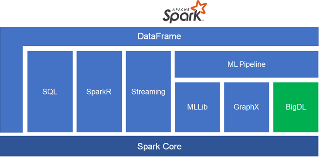