ML Model in Production: Real-world example of End-to-End ML Pipeline with TensorFlow Extended (TFX) & Apache Airflow on GCP

43 min readMar 29, 2022

Google Cloud Platform (GCP), TensorFlow Extended (TFX), Cloud Build, Cloud Storage, Cloud Functions, MLFlow, Vertex AI Pipeline, AI Platform, AI Platform Serving, Google Kubernetes Engine, KubeFlow Pipeline, Dataflow, Container Registry, MLFow Model Registry, Model Serving, Apache Beam, Cloud Composer, Airflow, DAG, CI/CD for TFX Pipeline, END-To-END example of real world Dataset using TFX Pipeline on Google Cloud Vertex AI platform

1. INTRODUCTION

A. Google Cloud Platform (GCP)

Cloud computing is an emerging technology being used in every area. Conventional organizations use IT infrastructure, which is not scalable according to their requirement. Organizations shift their workload to the cloud for enhancing their performance, scalability, and also for reduce cost. Google Cloud Platform (GCP) is a rising cloud computing platform with varieties of services like storage technologies, various kinds of databases, secure networking technologies, machine learning platforms, computing capabilities, and hosting of applications.

Advantages of hosting an application over cloud servers

Here are some of the cloud hosting benefits are:

a. Scalability 
b. Elasticity
c. Preconfigured OS images
d. High availability
e. Comparatively less time in provisioning on cloud
f. Persistence provided by a separate cloud storage facility
g. Cost-Efficient
h. Specific static IP address

Google Cloud Platform products and top services

Google Cloud Platform offered various services and products like Compute, Networking, Storage and Database, Machine Learning, Big data, and Identity and Access Management.

B. TFX (TensorFlow Extended)

TFX is a Google-production-scale machine learning toolkit based on TensorFlow for building and managing Machine Learning (ML) pipelines/workflows in a production environment. It provides a configuration framework and shared libraries to integrate common components needed to define, launch, and monitor your machine learning system. TFX pipelines let you orchestrate your ML workflow on several platforms, such as Apache Airflow, Apache Beam, and Kubeflow Pipelines.

The high-level architecture of the TFX pipeline on the Google Cloud Platform is shown below,

“TFX is a Google-production-scale machine learning (ML) platform based on TensorFlow. It provides a configuration framework and shared libraries to integrate common components needed to define, launch, and monitor your machine learning system.” according to the TFX User Guide.

TFX ML system on Google Cloud

In a production environment, the components of the system have to run at scale on a reliable platform. The following diagram shows how each step of the TFX ML pipeline runs using a managed service on Google Cloud, which ensures agility, reliability, and performance at a large scale.

TFX Standard Components
A TFX pipeline is a sequence of components that implement an ML pipeline that is specifically designed for scalable, high-performance machine learning tasks. That includes modeling, training, serving inference, and managing deployments to online, native mobile, and JavaScript targets.

This diagram illustrates the flow of data between TFX standard components:

High-level component overview of a machine learning platform.

The following are the TFX Pipeline Components:

Component: ExampleGen

It is the initial input component of a pipeline that ingests and optionally splits the input dataset. It takes raw data as input and generates TensorFlow examples, it can take many input formats (e.g. CSV files, TFRecord files with tf.Example, tf.SequenceExample and proto format, and results of BigQuery query). It also does split the examples for you into Train/Eval. It then passes the result to the StatisticsGen component.

The most common use case for splitting a Span is to split it into training and eval data.

Here is Span is a grouping of training examples. If your data is persisted on a filesystem, each Span may be stored in a separate directory. The semantics of a Span is not hardcoded into TFX; a Span may correspond to a day of data, an hour of data, or any other grouping that is meaningful to your task. Each Span can hold multiple versions of data and each version within a Span can further be subdivided into multiple Splits.

ExampleGen pipeline component can be used directly in deployment and requires little customization. For example:

examples = csv_input(os.path.join(data_root, 'simple'))
example_gen = CsvExampleGen(input_base=examples)

Custom input/output split

To customize the train/eval split ratio which ExampleGen will output, set the output_config for ExampleGen component. For example:

# Input has a single split 'input_dir/*'.
# Output 2 splits: train:eval=3:1.
output = proto.Output(
             split_config=example_gen_pb2.SplitConfig(splits=[
                 proto.SplitConfig.Split(name='train', hash_buckets=3),
                 proto.SplitConfig.Split(name='eval', hash_buckets=1)
             ]))
example_gen = CsvExampleGen(input_base=input_dir, output_config=output)

We can view an interactive widget of ExampleGen’s output. These outputs are called artifacts, and ExampleGen generally produces two artifacts — training examples and evaluation examples.

Component: StatisticsGen

The StatisticsGen component computes statistics over your dataset for data analysis, as well as for use in downstream components and also understanding its characteristics. It also comes with visualization tools. It uses the TensorFlow Data Validation library.

StatisticsGen takes as input the dataset we just ingested using ExampleGen.

A StatisticsGen pipeline component is typically very easy to deploy and requires little customization. Typical code looks like this:

compute_eval_stats = StatisticsGen(
      examples=example_gen.outputs['examples'],
      name='compute-eval-stats'
      )

For instance, Such a histogram helps determine the area we need to focus on to fix any data-related problems.

statistics_gen = StatisticsGen(input_data=example_gen.outputs.examples)

Using the StatsGen Component With a Schema, for the first run of a pipeline, the output of StatisticsGen will be used to infer a schema. However, on subsequent runs, you may have a manually curated schema that contains additional information about your data set.

user_schema_importer = Importer(
    source_uri=user_schema_dir, # directory containing only schema text proto
    artifact_type=standard_artifacts.Schema).with_id('schema_importer')

compute_eval_stats = StatisticsGen(
      examples=example_gen.outputs['examples'],
      schema=user_schema_importer.outputs['result'],
      name='compute-eval-stats'
      )

Component: SchemaGen

A SchemaGen pipeline component will automatically generate a schema by inferring types, categories, and ranges from the training data. TFX libraries that use the schema are TensorFlow Data Validation, TensorFlow Transform & TensorFlow Model Analysis.

In a typical TFX pipeline, SchemaGen generates a schema, which is consumed by the other pipeline components. However, the auto-generated schema is best-effort and only tries to infer basic properties of the data. For the initial schema generation, a SchemaGen pipeline component is typically very easy to deploy and requires little customization. Typical code looks like this:

schema_gen = tfx.components.SchemaGen(
    statistics=stats_gen.outputs['statistics'])

For the reviewed schema import, Add the ImportSchemaGen component to the pipeline to bring the reviewed schema definition into the pipeline.

schema_gen = tfx.components.ImportSchemaGen(
    schema_file='/some/path/schema.pbtxt')

In SchemaGen each feature in the dataset is represented, as well as the expected Type, Presence, Valency, and Domain.

Component: ExampleValidator

ExampleValidator takes the inputs and looks for problems in the data (missing values, 0 values that should not be 0) and report any anomalies. It can identify any anomalies among different classes in the example data by comparing data statistics computed by the StatisticsGen pipeline component against a schema. For example, it can:

i. perform validity checks by comparing data statistics against a schema that codifies expectations of the userii. detect training-serving skew by comparing training and serving data.iii. detect data drift by looking at a series of data.

An ExampleValidator pipeline component is typically very easy to deploy and requires little customization. Typical code looks like this:

example_validator = tfx.components.ExampleValidator(
    statistics=statistics_gen.outputs['statistics'],
    schema=schema_importer.outputs['result']
)
context.run(example_validator)
context.show(example_validator.outputs['anomalies'])

Component: Transform

The Transform TFX pipeline component performs feature engineering on tf.Examples are emitted from an ExampleGen component, using a data schema created by a SchemaGen component, and emits both a SavedModel as well as statistics on both pre-transform and post-transform data. For configuration of the Transform Component once preprocessing_fn is written, it needs to be defined in a python module that is then provided to the Transform component as an input. This module will be loaded by transform and the function name preprocessing_fn will be found and used by Transform to construct the preprocessing pipeline.

transform = tfx.components.Transform(
    examples=example_gen.outputs['examples'],
    schema=schema_importer.outputs['result'],
    module_file=os.path.abspath(TRANSFORM_MODULE_PATH),
)
context.run(transform, enable_cache=False)

For performing feature engineering on your dataset before it goes to your model Transform makes extensive use of TensorFlow Transform and It can also use as a part of the training process. Common feature transformations include:

a. Embedding: converting sparse features into dense features by finding a meaningful mapping from high-dimensional space to low dimensional space. b. Vocabulary generation: converting strings or other non-numeric features into integers by creating a vocabulary that maps each unique value to an ID number.c. Normalizing values: transforming numeric features so that they all fall within a similar range.d. Bucketization: converting continuous-valued features into categorical features by assigning values to discrete buckets.e. Enriching text features: producing features from raw data like tokens, n-grams, entities, sentiment, etc., to enrich the feature set.

The function name preprocessing_fn is defined below,

def preprocessing_fn(inputs):
  """tf.transform's callback function for preprocessing inputs.

  Args:
    inputs: map from feature keys to raw not-yet-transformed features.

  Returns:
    Map from string feature key to transformed feature operations.
  """
  outputs = {}
  for key in _DENSE_FLOAT_FEATURE_KEYS:
    # If sparse make it dense, setting nan's to 0 or '', and apply zscore.
    outputs[_transformed_name(key)] = transform.scale_to_z_score(
        _fill_in_missing(inputs[key]))

  for key in _VOCAB_FEATURE_KEYS:
    # Build a vocabulary for this feature.
    outputs[_transformed_name(
        key)] = transform.compute_and_apply_vocabulary(
            _fill_in_missing(inputs[key]),
            top_k=_VOCAB_SIZE,
            num_oov_buckets=_OOV_SIZE)

  for key in _BUCKET_FEATURE_KEYS:
    outputs[_transformed_name(key)] = transform.bucketize(
        _fill_in_missing(inputs[key]), _FEATURE_BUCKET_COUNT)

  for key in _CATEGORICAL_FEATURE_KEYS:
    outputs[_transformed_name(key)] = _fill_in_missing(inputs[key])

  # Was this passenger a big tipper?
  taxi_fare = _fill_in_missing(inputs[_FARE_KEY])
  tips = _fill_in_missing(inputs[_LABEL_KEY])
  outputs[_transformed_name(_LABEL_KEY)] = tf.where(
      tf.is_nan(taxi_fare),
      tf.cast(tf.zeros_like(taxi_fare), tf.int64),
      # Test if the tip was > 20% of the fare.
      tf.cast(
          tf.greater(tips, tf.multiply(taxi_fare, tf.constant(0.2))), tf.int64))

  return outputs

The execution results have shown below,

Component: Trainer

The Trainer TFX pipeline component trains a TensorFlow model. The Trainer TFX Pipeline takes:

a. tf.Examples used for training and eval.b. A user provided module file that defines the trainer logic.c. Protobuf definition of train args and eval args.d. (Optional) A data schema created by a SchemaGen pipeline component and optionally altered by the developer.e. (Optional) transform graph produced by an upstream Transform component.f. (Optional) pre-trained models used for scenarios such as warmstart.g. (Optional) hyperparameters, which will be passed to user module function. Details of the integration with Tuner can be found here.

Typical pipeline Domain Specific Language (DSL) code for the generic Trainer would look like this:

from tfx.components import Trainer

...

trainer = Trainer(
    module_file=module_file,
    examples=transform.outputs['transformed_examples'],
    transform_graph=transform.outputs['transform_graph'],
    train_args=trainer_pb2.TrainArgs(num_steps=10000),
    eval_args=trainer_pb2.EvalArgs(num_steps=5000))

The diagram below shows how training, serving & evaluating processes can happen in TFX Pipeline,

Trainer invokes a training module, which is specified in the module_file parameter. Instead of trainer_fn, a run_fn is required in the module file if the GenericExecutor is specified in the custom_executor_spec. The run_fn needs to handle the training part and output the trained model to the desired location given by FnArgs:

from tfx.components.trainer.fn_args_utils import FnArgs

def run_fn(fn_args: FnArgs) -> None:
  """Build the TF model and train it."""
  model = _build_keras_model()
  model.fit(...)
  # Save model to fn_args.serving_model_dir.
  model.save(fn_args.serving_model_dir, ...)

The trainer_fn was responsible for creating the model. Note that if the Transform component is not used in the pipeline, then the Trainer would take the examples from ExampleGen directly:

trainer = Trainer(
    module_file=module_file,
    examples=example_gen.outputs['examples'],
    schema=infer_schema.outputs['schema'],
    train_args=trainer_pb2.TrainArgs(num_steps=10000),
    eval_args=trainer_pb2.EvalArgs(num_steps=5000))

The Execution results will look like the below,

Component: Tuner

The Tuner component makes extensive use of the Python KerasTuner API for tuning hyperparameters.

The TFX Tuner tasks,

a. tf.Examples used for training and eval.b. A user provided module file (or module fn) that defines the tuning logic, including model definition, hyperparameter search space, objective etc.c. Protobuf definition of train args and eval args.d. (Optional) Protobuf definition of tuning args.e. (Optional) transform graph produced by an upstream Transform component.f. (Optional) A data schema created by a SchemaGen pipeline component and optionally altered by the developer.

A user module function tuner_fn with the following signature is required for Tuner:

...
from keras_tuner.engine import base_tuner

TunerFnResult = NamedTuple('TunerFnResult', [('tuner', base_tuner.BaseTuner),
                                             ('fit_kwargs', Dict[Text, Any])])

def tuner_fn(fn_args: FnArgs) -> TunerFnResult:
  """Build the tuner using the KerasTuner API.
  Args:
    fn_args: Holds args as name/value pairs.
      - working_dir: working dir for tuning.
      - train_files: List of file paths containing training tf.Example data.
      - eval_files: List of file paths containing eval tf.Example data.
      - train_steps: number of train steps.
      - eval_steps: number of eval steps.
      - schema_path: optional schema of the input data.
      - transform_graph_path: optional transform graph produced by TFT.
  Returns:
    A namedtuple contains the following:
      - tuner: A BaseTuner that will be used for tuning.
      - fit_kwargs: Args to pass to tuner's run_trial function for fitting the
                    model , e.g., the training and validation dataset. Required
                    args depend on the above tuner's implementation.
  """
  ...

The trainer can take Tuner’s output hyperparameters as input and utilize them in its user module code. The pipeline definition looks like this:

...
tuner = Tuner(
    module_file=module_file,  # Contains `tuner_fn`.
    examples=transform.outputs['transformed_examples'],
    transform_graph=transform.outputs['transform_graph'],
    train_args=trainer_pb2.TrainArgs(num_steps=20),
    eval_args=trainer_pb2.EvalArgs(num_steps=5))

trainer = Trainer(
    module_file=module_file,  # Contains `run_fn`.
    examples=transform.outputs['transformed_examples'],
    transform_graph=transform.outputs['transform_graph'],
    schema=schema_gen.outputs['schema'],
    # This will be passed to `run_fn`.
    hyperparameters=tuner.outputs['best_hyperparameters'],
    train_args=trainer_pb2.TrainArgs(num_steps=100),
    eval_args=trainer_pb2.EvalArgs(num_steps=5))
...

You might not want to tune the hyperparameters every time you retrain your model. Once you have used Tuner to determine a good set of hyperparameters, you can remove Tuner from your pipeline and use ImporterNode it to import the Tuner artifact from a previous training run to feed to Trainer.

hparams_importer = Importer(
    # This can be Tuner's output file or manually edited file. The file contains
    # text format of hyperparameters (keras_tuner.HyperParameters.get_config())
    source_uri='path/to/best_hyperparameters.txt',
    artifact_type=HyperParameters,
).with_id('import_hparams')

trainer = Trainer(
    ...
    # An alternative is directly use the tuned hyperparameters in Trainer's user
    # module code and set hyperparameters to None here.
    hyperparameters = hparams_importer.outputs['result'])

Parallel Tuning

In parallel tuning, multiple trials are executed in parallel. In the search the function of the tuner, trials will be run in sequence instead of in parallel. To support parallel tuning, we need to launch multiple tuners (the tuner here refers to the one in the KerasTuner library, not the TFX Tuner component) and have an optimization service for managing the state of the tuning algorithm, with which oracle of each tuner communicates, and retrieves the trials for each tuner.

The number of parallel tuners can be passed to the component by the TuneArgs as shown below:

# Args specific to tuning.
message TuneArgs {
  # Number of trials to run in parallel.
  # Each trial will be trained and evaluated by separate worker jobs.
  int32 num_parallel_trials = 1;
}

class TunerSpec(ComponentSpec):

  PARAMETERS = {
    ...
    'tune_args': ExecutionParameter(type=tuner_pb2.TuneArgs),

Tuning on Google Cloud Platform (GCP): Below is a code snippet that shows how to use CloudTuner. Notice that configuration to CloudTuner requires items that are specific to GCP, such as the project_id and region.

...
from tensorflow_cloud import CloudTuner

...
def tuner_fn(fn_args: FnArgs) -> TunerFnResult:
  """An implementation of tuner_fn that instantiates CloudTuner."""

  ...
  tuner = CloudTuner(
      _build_model,
      hyperparameters=...,
      ...
      project_id=...,       # GCP Project ID
      region=...,           # GCP Region where Vizier service is run.
  )

  ...
  return TuneFnResult(
      tuner=tuner,
      fit_kwargs={...}
  )

Google Cloud AI Platform extension Tuner

The Google Cloud AI Platform extension Tuner component provides the ability to run parallel tuning, using an AI Platform Training Job as a distributed worker flock manager. TuneArgs is the configuration given to this component.

tuner = google_cloud_ai_platform.Tuner(
    ...   # Same kwargs as the above stock Tuner component.
    tune_args=proto.TuneArgs(num_parallel_trials=3),  # 3-worker parallel
    custom_config={
        # Configures Cloud AI Platform-specific configs . For for details, see
        # https://cloud.google.com/ai-platform/training/docs/reference/rest/v1/projects.jobs#traininginput.
        TUNING_ARGS_KEY:
            {
                'project': ...,
                'region': ...,
                # Configuration of machines for each master/worker in the flock.
                'masterConfig': ...,
                'workerConfig': ...,
                ...
            }
    })
...

Below shows the workflow for in-process tuning and Cloud tuning.

Component: Evaluator

The Evaluator TFX pipeline component performs deep analysis on the training results for your models, to help you understand how your model performs on subsets of your data. The Evaluator also helps you validate your exported models, ensuring that they are “good enough” to be pushed to production.

Typical code looks like this:

import tensorflow_model_analysis as tfma
...

# For TFMA evaluation

eval_config = tfma.EvalConfig(
    model_specs=[
        # This assumes a serving model with signature 'serving_default'. If
        # using estimator based EvalSavedModel, add signature_name='eval' and
        # remove the label_key. Note, if using a TFLite model, then you must set
        # model_type='tf_lite'.
        tfma.ModelSpec(label_key='<label_key>')
    ],
    metrics_specs=[
        tfma.MetricsSpec(
            # The metrics added here are in addition to those saved with the
            # model (assuming either a keras model or EvalSavedModel is used).
            # Any metrics added into the saved model (for example using
            # model.compile(..., metrics=[...]), etc) will be computed
            # automatically.
            metrics=[
                tfma.MetricConfig(class_name='ExampleCount'),
                tfma.MetricConfig(
                    class_name='BinaryAccuracy',
                    threshold=tfma.MetricThreshold(
                        value_threshold=tfma.GenericValueThreshold(
                            lower_bound={'value': 0.5}),
                        change_threshold=tfma.GenericChangeThreshold(
                            direction=tfma.MetricDirection.HIGHER_IS_BETTER,
                            absolute={'value': -1e-10})))
            ]
        )
    ],
    slicing_specs=[
        # An empty slice spec means the overall slice, i.e. the whole dataset.
        tfma.SlicingSpec(),
        # Data can be sliced along a feature column. In this case, data is
        # sliced along feature column trip_start_hour.
        tfma.SlicingSpec(feature_keys=['trip_start_hour'])
    ])

# The following component is experimental and may change in the future. This is
# required to specify the latest blessed model will be used as the baseline.
model_resolver = Resolver(
      strategy_class=dsl.experimental.LatestBlessedModelStrategy,
      model=Channel(type=Model),
      model_blessing=Channel(type=ModelBlessing)
).with_id('latest_blessed_model_resolver')

model_analyzer = Evaluator(
      examples=examples_gen.outputs['examples'],
      model=trainer.outputs['model'],
      baseline_model=model_resolver.outputs['model'],
      # Change threshold will be ignored if there is no baseline (first run).
      eval_config=eval_config)

The evaluator produces an EvalResult (and optionally a ValidationResult if validation was used) that can be loaded using TFMA. The following is an example of code:

eval_config = tfma.EvalConfig(
    model_specs=[
                 tfma.ModelSpec(
                     signature_name="serving_default",
                     preprocessing_function_names=['tft_layer'],
                     label_key="Purchased",
                 )
    ],
    metrics_specs = [
                     tfma.MetricsSpec(
                         per_slice_thresholds={
                             "binary_accuracy": tfma.PerSliceMetricThresholds(
                                 thresholds=[
                                             tfma.PerSliceMetricThreshold(
                                                 slicing_specs=[tfma.SlicingSpec()],
                                                 threshold=tfma.MetricThreshold(
                                                     value_threshold=tfma.GenericValueThreshold(
                                                         lower_bound={"value":0.7}
                                                     ),
                                                     change_threshold=tfma.GenericChangeThreshold(
                                                         direction=tfma.MetricDirection.HIGHER_IS_BETTER,
                                                         absolute={"value": -1e-10},
                                                     ),
                                                 ),
                                             )
                                 ]
                             ),
                         }
                     )
    ],
    slicing_specs=[
                   tfma.SlicingSpec(),
                   tfma.SlicingSpec(feature_keys=["Gender"])
    ]
)model_resolver = tfx.dsl.Resolver(
    strategy_class=tfx.dsl.experimental.LatestBlessedModelStrategy,
    model=tfx.dsl.Channel(type=tfx.types.standard_artifacts.Model),
    model_blessings=tfx.dsl.Channel(type=tfx.types.standard_artifacts.ModelBlessing),
).with_id("latest_blessed_model_resolver")

context.run(model_resolver)

The ExecutionResults is shown below,

evaluator = tfx.components.Evaluator(
    examples=example_gen.outputs["examples"],
    model=trainer.outputs["model"],
    eval_config=eval_config,
    baseline_model=model_resolver.outputs["model"],
)

context.run(evaluator, enable_cache=False)

The ExecutionResults is shown below,

Component: InfraValidator

InfraValidator checks the model is actually servable from the infrastructure and prevents the bad models from being pushed. If Evaluator is to guarantee the performance of the model, InfraValidator is to guarantee the model is mechanically fine and prevents bad models from being pushed.

InfraValidator is defined next to an Evaluator component, and its output is fed to a Pusher. If InfraValidator fails, the model will not be pushed.

evaluator = Evaluator(
    model=trainer.outputs['model'],
    examples=example_gen.outputs['examples'],
    baseline_model=model_resolver.outputs['model'],
    eval_config=tfx.proto.EvalConfig(...)
)

infra_validator = InfraValidator(
    model=trainer.outputs['model'],
    serving_spec=tfx.proto.ServingSpec(...)
)

pusher = Pusher(
    model=trainer.outputs['model'],
    model_blessing=evaluator.outputs['blessing'],
    infra_blessing=infra_validator.outputs['blessing'],
    push_destination=tfx.proto.PushDestination(...)
)

The choice for serving binary and the serving platform is made by specifying a oneof block of the ServingSpec. For example to use TensorFlow Serving binary running on the Kubernetes cluster, tensorflow_serving and kubernetes the field should be set.

infra_validator=InfraValidator(
    model=trainer.outputs['model'],
    serving_spec=tfx.proto.ServingSpec(
        tensorflow_serving=tfx.proto.TensorFlowServing(
            tags=['latest']
        ),
        kubernetes=tfx.proto.KubernetesConfig()
    )
)

Optional configuration to adjust the infra validation criteria or workflow.

infra_validator=InfraValidator(
    model=trainer.outputs['model'],
    serving_spec=tfx.proto.ServingSpec(...),
    validation_spec=tfx.proto.ValidationSpec(
        # How much time to wait for model to load before automatically making
        # validation fail.
        max_loading_time_seconds=60,
        # How many times to retry if infra validation fails.
        num_tries=3
    )
)

Depending on the configuration, infra validation is done in one of the following modes:

LOAD_ONLY mode: checking whether the model was successfully loaded in the serving infrastructure or not. OR
LOAD_AND_QUERY mode: LOAD_ONLY mode plus sending some sample requests to check if the model is capable of serving inferences.

In order to use LOAD_AND_QUERY mode, it is required to specify both request_spec execution properties as well as examples input channels in the component definition.

infra_validator = InfraValidator(
    model=trainer.outputs['model'],
    # This is the source for the data that will be used to build a request.
    examples=example_gen.outputs['examples'],
    serving_spec=tfx.proto.ServingSpec(
        # Depending on what kind of model server you're using, RequestSpec
        # should specify the compatible one.
        tensorflow_serving=tfx.proto.TensorFlowServing(tags=['latest']),
        local_docker=tfx.proto.LocalDockerConfig(),
    ),
    request_spec=tfx.proto.RequestSpec(
        # InfraValidator will look at how "classification" signature is defined
        # in the model, and automatically convert some samples from `examples`
        # artifact to prediction RPC requests.
        tensorflow_serving=tfx.proto.TensorFlowServingRequestSpec(
            signature_names=['classification']
        ),
        num_examples=10  # How many requests to make.
    )
)

Component: Pusher

The Pusher component is used to push a validated model to a deployment target during model training or re-training. Before the deployment, Pusher relies on one or more blessings from other validation components to decide whether to push the model or not.

Pusher TFX Pipeline has different model deployment options:

Filesystem (TensorFlow Lite, TensorFlow JS)
TensorFlow Serving

It can be configured to block deployment on the outcome of model validation. A Pusher component consumes a trained model in SavedModel format, and produces the same SavedModel, along with versioning metadata.

Typical code looks like this:

pusher = Pusher(
  model=trainer.outputs['model'],
  model_blessing=evaluator.outputs['blessing'],
  infra_blessing=infra_validator.outputs['blessing'],
  push_destination=tfx.proto.PushDestination(
    filesystem=tfx.proto.PushDestination.Filesystem(
        base_directory=serving_model_dir)
  )
)

InfraValidator can also produce InfraBlessing artifact containing a model with a warmup, and Pusher can push it just like a Model artifact.

infra_validator = InfraValidator(
    ...,
    # make_warmup=True will produce a model with warmup requests in its
    # 'blessing' output.
    request_spec=tfx.proto.RequestSpec(..., make_warmup=True)
)

pusher = Pusher(
    # Push model from 'infra_blessing' input.
    infra_blessing=infra_validator.outputs['blessing'],
    push_destination=tfx.proto.PushDestination(...)
)

The ExecutionResults will look like this:

Component: BulkInferrer

BulkInferrer performs batch processing on a model with unlabelled inference requests tf.Examples. It is typically deployed after an Evaluator component to perform inference with a validated model, or after a Trainer, component to directly perform inference on the exported model.

The Code is as below:

bulk_inferrer = BulkInferrer(
    examples=examples_gen.outputs['examples'],
    model=trainer.outputs['model'],
    model_blessing=evaluator.outputs['blessing'],
    data_spec=bulk_inferrer_pb2.DataSpec(),
    model_spec=bulk_inferrer_pb2.ModelSpec()
)

TFX Pipeline

All components can be used together to create a pipeline. The following code snippet illustrates how to create a TFX pipeline:

i. Define the components, their input, and output

ii. Create a runner (e.g. Airflow) that will execute the pipeline

iii. Pass the list of components to the runner to initiate the pipeline execution

Here is the code example:

def _create_pipeline():
  """Implements a TFX pipeline."""
  csv_data = csv_input(os.path.join(data_root, 'simple'))
  example_gen = CsvExampleGen(input=csv_data)

  statistics_gen = StatisticsGen(examples=example_gen.outputs['examples'])
  infer_schema = SchemaGen(statistics=statistics_gen.outputs['statistics'])
  validate_stats = ExampleValidator(statistics=statistics_gen.output['statistics'], schema=infer_schema.outputs['schema'])

  # Performs feature engineering
  transform = Transform(examples=example_gen.outputs['examples'], schema=infer_schema.outputs['schema'], module_file=_taxi_module_file)

  trainer = Trainer(...)
  model_analyzer = Evaluator(examples=example_gen.outputs['examples'], model=trainer.outputs['model'])
  model_validator = ModelValidator(examples=example_gen.outputs['examples'], model=trainer.outputs['model'])
  pusher = Pusher(model=..., model_blessing=..., serving_model_dir=...)

  return [example_gen, statistics_gen, infer_schema, validate_stats, transform, trainer, model_analyzer, model_validator, pusher]

result = AirflowDAGRunner(_airflow_config).run(_create_pipeline())

TFX components at run time

The TFX Pipeline component is executed in three phases

i. First, the Driver uses the component specification to retrieve the required artifacts from the metadata store and pass them into the component.

ii. Next, the Executor performs the component’s work.

iii. Then the Publisher uses the component specification and the results from the executor to store the component’s outputs in the metadata store.

The modifications to the Driver and Publisher should be necessary only if you want to change the interaction between your pipeline’s components and the metadata store.

A TFX pipeline is a sequence of components connected by channels in a directed acyclic graph (DAG) of artifact dependencies as shown below,

TFX Libraries

TFX provides several Python packages that are the libraries that are used to create pipeline components. TFX libraries include the following:

i. TensorFlow Data Validation (TFDV)

Tensorflow Data Validation (TFDV) is a library for analyzing and validating machine learning data. It is designed to be highly scalable and to work well with TensorFlow and TFX. It has a schema viewer, scalable calculations, and dataset comparison.

TensorFlow Data Validation provides tools for visualizing the distribution of feature values. By examining these distributions in a Jupyter notebook using Facets you can catch common problems with data.

TFDV includes the following:

a. Scalable calculation of summary statistics of training and test data.b. Integration with a viewer for data distributions and statistics, as well as faceted comparison of pairs of datasets (Facets).c. Automated data-schema generation to describe expectations about data like required values, ranges, and vocabularies.d. A schema viewer to help you inspect the schema.e. Anomaly detection to identify anomalies, such as missing features, out-of- range values, or wrong feature types, to name a few.f. An anomalies viewer so that you can see what features have anomalies and learn more in order to correct them.

ii. Tensorflow Transform (TFT)

TensorFlow Transform (TFT) is a library for preprocessing data with TensorFlow.

a. Normalize an input value by mean and standard deviation.b. Convert strings to integers by generating a vocabulary over all input values.c. Convert floats to integers by assigning them to buckets based on the observed data distribution.

TensorFlow has built-in support for manipulations on a single example or a batch of examples. tf.Transform extends these capabilities to support full passes over the example data.

The output of tf.Transform is exported as a TensorFlow graph to use for training and serving. Using the same graph for both training and serving can prevent skew since the same transformations are applied in both stages.

In the preprocessing function below, NUMERICAL_COLUMNS and CATEGORICAL_COLUMNS are lists that contain the names of the numeric and categorical columns:

def preprocessing_fn(inputs):
  """Preprocess input columns into transformed columns."""
  # Since we are modifying some features and leaving others unchanged, we
  # start by setting `outputs` to a copy of `inputs.
  outputs = inputs.copy()

  # Scale numeric columns to have range [0, 1].
  for key in NUMERIC_FEATURE_KEYS:
    outputs[key] = tft.scale_to_0_1(outputs[key])

  for key in OPTIONAL_NUMERIC_FEATURE_KEYS:
    # This is a SparseTensor because it is optional. Here we fill in a default
    # value when it is missing.
      sparse = tf.sparse.SparseTensor(outputs[key].indices, outputs[key].values,
                                      [outputs[key].dense_shape[0], 1])
      dense = tf.sparse.to_dense(sp_input=sparse, default_value=0.)
    # Reshaping from a batch of vectors of size 1 to a batch to scalars.
    dense = tf.squeeze(dense, axis=1)
    outputs[key] = tft.scale_to_0_1(dense)

  # For all categorical columns except the label column, we generate a
  # vocabulary but do not modify the feature.  This vocabulary is instead
  # used in the trainer, by means of a feature column, to convert the feature
  # from a string to an integer id.
  for key in CATEGORICAL_FEATURE_KEYS:
    tft.vocabulary(inputs[key], vocab_filename=key)

  # For the label column we provide the mapping from string to index.
  initializer = tf.lookup.KeyValueTensorInitializer(
      keys=['>50K', '<=50K'],
      values=tf.cast(tf.range(2), tf.int64),
      key_dtype=tf.string,
      value_dtype=tf.int64)
  table = tf.lookup.StaticHashTable(initializer, default_value=-1)

  outputs[LABEL_KEY] = table.lookup(outputs[LABEL_KEY])

  return outputs

The diagram below is a good visual of how the last 2 feature works:

iii. TensorFlow

Tensorflow is used for training models with TFX. It ingests training data and modeling code and creates a SavedModel result. It also integrates a feature engineering pipeline created by TensorFlow Transform for preprocessing input data.

KerasTuner is used for tuning hyperparameters for the model. Hyperparameters are of two types:

a. Model hyperparameters:

Model hyperparameter influences model selection such as the number and width of hidden layers

b. Algorithm hyperparameters

Algorithm hyperparameters influence the speed and quality of the learning algorithm such as the learning rate for Stochastic Gradient Descent (SGD) and the number of nearest neighbors for a k Nearest Neighbors (KNN) classifier.

We can visualize ML experimentation integrated with TFX on Tensorboard as shown below,

iv. Tensorflow Model Analysis (TFMA)

Tensorflow Model Analysis (TFMA) Library for evaluating TensorFlow models. It is used along with TensorFlow to create an EvalSavedModel, which becomes the basis for its analysis. It allows users to evaluate their models on large amounts of data in a distributed manner, using the same metrics defined in their trainer. These metrics can be computed over different slices of data and visualized in Jupyter notebooks.

The following uses tfma.run_model_analysis to perform an evaluation on a serving model.

# Run in a Jupyter Notebook.
from google.protobuf import text_format

eval_config = text_format.Parse("""
  ## Model information
  model_specs {
    # This assumes a serving model with a "serving_default" signature.
    label_key: "label"
    example_weight_key: "weight"
  }
  ## Post export metric information
  metrics_specs {
    # This adds AUC and as a post training metric. If the model has built in
    # training metrics which also contains AUC, this metric will replace it.
    metrics { class_name: "AUC" }
    # ... other post training metrics ...

    # Plots are also configured here...
    metrics { class_name: "ConfusionMatrixPlot" }
  }
  ## Slicing information
  slicing_specs {}  # overall slice
  slicing_specs {
    feature_keys: ["age"]
  }
""", tfma.EvalConfig())

eval_shared_model = tfma.default_eval_shared_model(
    eval_saved_model_path='/path/to/saved/model', eval_config=eval_config)

eval_result = tfma.run_model_analysis(
    eval_shared_model=eval_shared_model,
    eval_config=eval_config,
    # This assumes your data is a TFRecords file containing records in the
    # tf.train.Example format.
    data_location='/path/to/file/containing/tfrecords',
    output_path='/path/for/output')

tfma.view.render_slicing_metrics(eval_result)

To perform model validation against a candidate and baseline, update the config to include a threshold setting and pass two models to tfma.run_model_analysis.

# Run in a Jupyter Notebook.
from google.protobuf import text_formateval_config = text_format.Parse("""
  ## Model information
  model_specs {
    # This assumes a serving model with a "serving_default" signature.
    label_key: "label"
    example_weight_key: "weight"
  }
  ## Post export metric information
  metrics_specs {
    # This adds AUC and as a post training metric. If the model has built in
    # training metrics which also contains AUC, this metric will replace it.
    metrics {
      class_name: "AUC"
      threshold {
        value_threshold {
          lower_bound { value: 0.9 }
        }
        change_threshold {
          direction: HIGHER_IS_BETTER
          absolute { value: -1e-10 }
        }
      }
    }
    # ... other post training metrics ...    # Plots are also configured here...
    metrics { class_name: "ConfusionMatrixPlot" }
  }
  ## Slicing information
  slicing_specs {}  # overall slice
  slicing_specs {
    feature_keys: ["age"]
  }
""", tfma.EvalConfig())eval_shared_models = [
  tfma.default_eval_shared_model(
      model_name=tfma.CANDIDATE_KEY,
      eval_saved_model_path='/path/to/saved/candiate/model',
      eval_config=eval_config),
  tfma.default_eval_shared_model(
      model_name=tfma.BASELINE_KEY,
      eval_saved_model_path='/path/to/saved/baseline/model',
      eval_config=eval_config),
]output_path = '/path/for/output'eval_result = tfma.run_model_analysis(
    eval_shared_models,
    eval_config=eval_config,
    # This assumes your data is a TFRecords file containing records in the
    # tf.train.Example format.
    data_location='/path/to/file/containing/tfrecords',
    output_path=output_path)tfma.view.render_slicing_metrics(eval_result)
tfma.load_validation_result(output_path)

These metrics can be computed over different slices of data and visualized in Jupyter notebooks as shown below,

The diagram is shown below comparing TFMA to Tensorboard:

v. TensorFlow Metadata (TFMD)

Tensorflow Metadata (TFMD) provides standard representations for metadata that are useful when training machine learning models with TensorFlow. The metadata may be produced by hand or automatically during input data analysis, and maybe consumed for data validation, exploration, and transformation.

The metadata serialization formats include:

i. A schema describing tabular data (e.g., tf.Examples).

ii. A collection of summary statistics over such datasets.

iii. A problem statement quantifying the objectives of a model.

vi. Machine Learning Metadata (MLMD)

ML Metadata (MLMD) is a library for recording and retrieving metadata associated with ML developer and data scientist workflows. MLMD is an integral part of TensorFlow Extended (TFX) but is designed so that it can be used independently. The ML metadata store is a “store” for ML model-related metadata. It is a place where you can get anything you need when it comes to any and every ML model you build and deploy.

A high-level overview of the various components that are part of MLMD as shown below,

It is an open-source pipeline-first ML metadata store that powers TensorFlow Extended (TFX) and Kubelfow.

Some benefits of MLMD:

i. Recurse back to see what data went into a modelii. See all Models trained from a specific datasetiii. Show a DAG of all executions and their input and output artifactsiv. Compare results from two experiments

An end to end ML pipeline might look like this with TFX libraries:

TFX pipelines use ML Metadata for artifact management and an orchestrator for sequential component execution as shown below,

ML Metadata in Action: i. Register ArtifactTypes ii. Register ExecutionTypes iii. Create Dataset Artifact iv. Create Execution for Trainer v. Reading Dataset and Record input event vi. Train Model and Create SavedModel Artifact vii. Write SavedModel and record output event viii. Mark Execution completed
ix. Annotate the experiment with a context

There are 3 specialized features nodes for advanced Metadata operation in TFX Pipeline:

i. PipelineNodes: They’re special-purpose classes for conducting advanced metadata operations like querying current ML metadata using artifact properties.

ii. ImporterNode: It is a specialized features node that integrates an external resource into the ML metadata library so that downstream nodes may use the registered artifacts as input, which is the most popular pipeline node. This node’s primary mission is to bring external artifacts, such as a schema, into the TFX pipeline for usage by the transform in trainer components.

iii. ResolverNode: The model resolver is only required if performing model validation in addition to evaluation. In this case, we validate against the latest blessed model. If no model has been blessed before (as in this case) the evaluator will make our candidate the first blessed model.

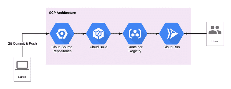
C. Cloud Build

For continuously building, testing, and deploying containers the Cloud Build is a managed service on Google Cloud Platform infrastructure that allows you. It also lets you build software quickly across all languages. It works across multiple environments such as VMs, serverless, Kubernetes, or Firebase.

Cloud Build also helps for automatically building and deploying containers into Cloud Run when changes are pushed to the CSR repository.

After enabling Cloud Build API on GCP it will look like the below,

D. Cloud Storage

Google Cloud Storage is the object storage service offered by Google Cloud. It provides some very interesting out-of-the-box features such as object versioning or fine-grain permissions (per object or bucket), that can make development easy and help reduce operational overheads. Google Cloud Storage serves as the foundation of several different services.

The highest level of availability and performance within a single region is ideal for compute, analytics, and machine learning workloads in a particular region. Cloud Storage is also strongly consistent, giving you confidence and accuracy in analytics workloads.

After enabling Cloud Storage API, we can see Cloud Storage Dashboard on GCP as shown below,

E. Cloud Functions, App Engine & Cloud Run

Google Cloud Functions scales as needed and integrates with Google Cloud’s operations suite (such as Cloud Logging) out of the box. Event-driven solutions that extend to Google and 3rd party services are a good fit for cloud functions, as well as ones that need to scale quickly. Cloud Functions support individualized services. For example, if you are saving or extracting data from a database, posting a file, or doing simple data validation, then using Cloud Functions is an appropriate choice.

The Cloud Function API on GCP as shown below,

Google App Engine is mainly a platform a service that allows a user to develop and execute applications through the Google framework, thus removing the need for expensive acquisition and maintenance of a database, as it is managed by Google. App Engine supports many different services within a single application.

The figure below shows the structure of the Google app engine which includes client capabilities containing the tools available for a user, cloud computing services, and the support services in place.

Cloud Run can scale stateless containers and leverages Google Kubernetes Engine. If you need a serverless option that needs an application to run in a stateless container, Cloud Run may be the best choice for this kind of deployment. It is fully managed, and the pricing is based only on resources consumed.

When it comes to managing servers, problems abound:

i. Provisioning servers

ii. Scaling servers up/down to meet demands

iii. Overpaying when more resources are allocated than necessary

Cloud Run API on GCP as shown below,

The figure below shows how to choose an application between Cloud Function, App Engine & Cloud Run,

F. MLFlow

MLflow is a platform to streamline machine learning development, including tracking experiments, packaging code into reproducible runs, and sharing and deploying models. MLflow offers a set of lightweight APIs that can be used with any existing machine learning application or library (TensorFlow, PyTorch, XGBoost, etc).

MLflow’s current components are:

a. MLflow Tracking: An API to log parameters, code, and results in machine learning experiments and compare them using an interactive UI.

b. MLflow Projects: A code packaging format for reproducible runs using Conda and Docker, so you can share your ML code with others.

c. MLflow Models: A model packaging format and tools that let you easily deploy the same model (from any ML library) to batch and real-time scoring on platforms such as Docker, Apache Spark, Azure ML, and AWS SageMaker .You can add metadata to your MLflow models, including Model Signature & Model Input Example.

d. Model Registry: A centralized model store, set of APIs, and UI, to collaboratively manage the full lifecycle of MLflow Models.

The registry provides model lineage, model versioning, annotations, and stage transitions. The below figure shows that the Model Registry workflow UI,

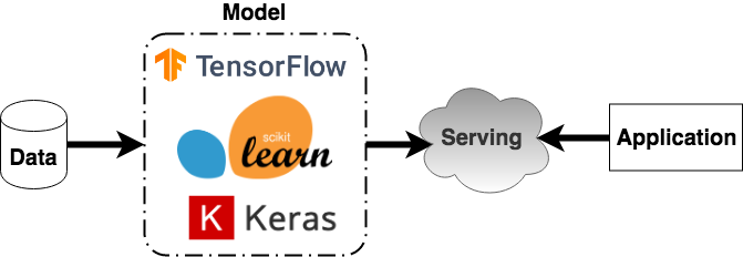
G. Model Serving

Model Serving

Once a model is trained it needs to be made available to other components — a process usually called serving. The goal is to provide a way to query the model, getting outputs for a certain set of inputs.

Serverless model serving example as shown below,

Google Cloud Platform (GCP) provides multiple ways for deploying inference in the cloud. There are the following methods for deploying the model: i. Compute Engine cluster with TF serving ii. Cloud AI Platform Predictions, iii. Cloud Functions.

TensorFlow Serving
TensorFlow Serving is a flexible, high-performance serving system for machine learning models, designed for production environments. TensorFlow Serving makes it easy to deploy new algorithms and experiments while keeping the same server architecture and APIs. TensorFlow Serving provides out-of-the-box integration with TensorFlow models but can be easily extended to serve other types of models and data.

This approach has the following advantages:

i. Great response time as the model will be loaded in the memory

ii. Economy of scale, meaning the cost per run will decrease significantly when you have a lot of requests

H. Vertex AI Pipeline, AI Platform & AI Platform Serving

Vertex AI Pipeline

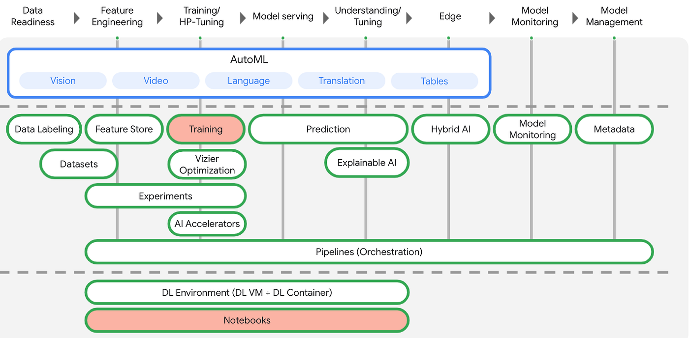
Vertex AI Pipelines helps you to automate, monitor, and govern your ML systems by orchestrating your ML workflow in a serverless manner and storing your workflow’s artifacts using Vertex ML Metadata. We can see Google’s Vertex AI Platform service as shown below,

Google has promoted a nice diagram resuming the overall components offered by Vertex AI. The MLOps overview on Vertex AI Pipeline as shown below,

To orchestrate your ML workflow on Vertex AI Pipelines, you must first describe your workflow as a pipeline. ML pipelines are portable and scalable ML workflows that are based on containers. Vertex AI brings a greater focus on machine learning operations or MLOps. The company says that Vertex AI can reduce the number of lines of code that data scientists and ML engineers have to write by up to 80%.

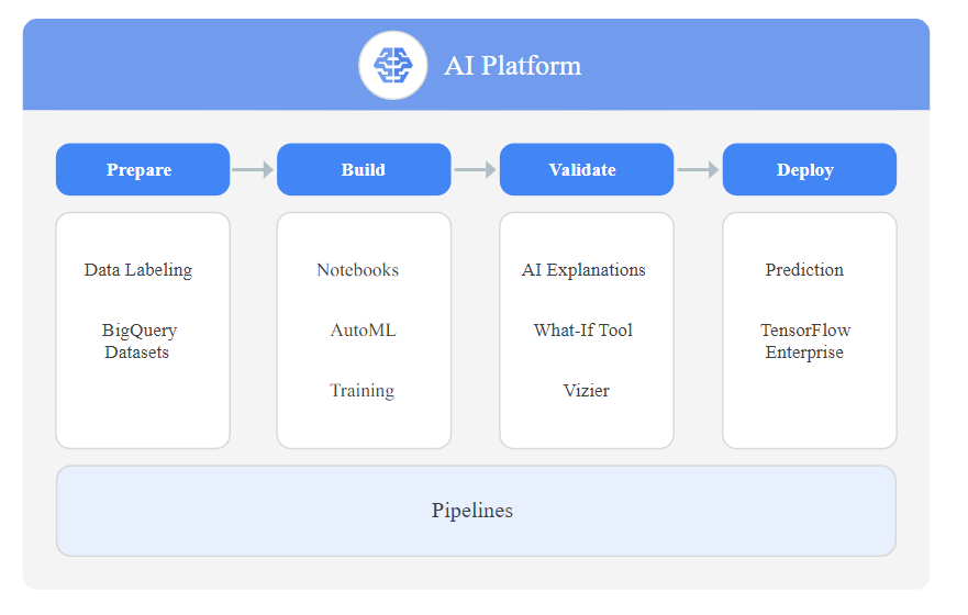
AI Platform

The AI Platform to train your machine learning models at scale, to host your trained model in the cloud, and use your model to make predictions about new data. AI Platform is a suite of services on Google Cloud specifically targeted at the building, deploying, and managing machine learning models in the cloud.

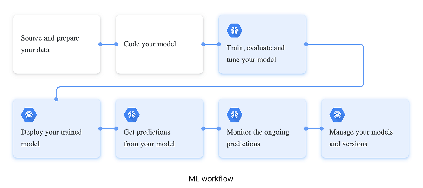
Cloud AI Platform Services

AI Platform offers a suite of services, designed to support the activities seen in a typical ML workflow. Where AI Platform fits in the ML workflow. The diagram below gives a high-level overview of the stages in an ML workflow. The blue-filled boxes indicate where AI Platform provides managed services and APIs:

ML Ops is the practice of deploying robust, repeatable, and scalable ML pipelines to manage your models. AI Platform offers a number of services to assist with these pipelines. The AI Platform Pipelines provide support for creating ML pipelines, using either Kubeflow Pipelines or TensorFlow Extended (TFX) and Continuous evaluation helps you monitor the performance of your models and provides continual feedback on how your models are performing over time.

The AI Platform Serving overview is shown below,

I. Container Registry, Google Kubernetes Engine & KubeFlow Pipeline

Container Registry

Container Registry is a single place for the team to manage Docker images, perform vulnerability analysis, and decide who can access what with fine-grained access control. Existing CI/CD integrations let you set up fully automated Docker pipelines to get fast feedback.

GCP Serverless CI/CD Pipeline Architecture as shown below,

The Artifact Registry is the next generation of the Container Registry. Artifact Registry improves and extends upon the existing capabilities of Container Registry, such as customer-managed encryption keys, VPC-SC support, Pub/Sub notifications, and more, providing a foundation for major upgrades in security, scalability, and control. While Container Registry is still available and will continue to be supported as a Google Enterprise API.

Google Kubernetes Engine

Google Kubernetes Engine (GKE), a managed service used for containerized applications for their orchestration is used to deploy simple or complex web applications, complex tasks, or even to run ML and AI infrastructure based on Kubernetes. We can perform some operations on it are like i. To Create a Kubernetes object, i.e., pods, ReplicaSet, Deployment Services, jobs, and many others ii. We can update containers, iii. We can resize the Replicaset. We can interact with gcloud using CLI (Local) or using the google cloud shell. Kubernetes Architecture Overview.

A Kubernetes cluster consists of a set of worker machines, called nodes, that run containerized applications. Every cluster has at least one worker node. The worker node(s) host the Pods which are the components of the application workload. The control plane manages the worker nodes and the Pods in the cluster. In production environments, the control plane usually runs across multiple computers and a cluster usually runs multiple nodes, providing fault-tolerance and high availability. The figure below shows the structure of GKE on the Google Cloud Platform,

To create Your First Cluster Using GKE firstly you need to login into your account then open the Google Cloud Platform console. On the left side, you have an option name Kubernetes Engine under the compute category.

Kubernetes objects are persistent entities in the Kubernetes system. Kubernetes uses these entities to represent the state of your cluster. Specifically, they can describe:

i. What containerized applications are running (and on which nodes)

ii. The resources available to those applications

iii. The policies around how those applications behave, such as restart policies, upgrades, and fault-tolerance

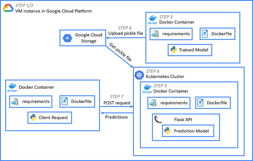
Machine Learning Training and Deployment of end-to-end architecture on GKE as shown below,

The difference between Kubernetes and Docker Swarm as shown below,

Kubeflow is the cloud-native platform for machine learning operations like pipelines, training, and deployment. Kubeflow builds on Kubernetes as a system for deploying, scaling and managing complex systems.

Using the Kubeflow configuration interfaces you can specify the ML tools required for your workflow. Then you can deploy the workflow to various clouds, local, and on-premises platforms for experimentation and for production use.

Kubeflow supports a TensorFlow Serving container to export trained TensorFlow models to Kubernetes. Training multiple models in Kubeflow pipeline as shown below,

Kubeflow Pipelines provides a new method of generating visualizations. This image comes from the Kubeflow Pipelines UI.

The Kubeflow Pipelines UI offers built-in support for several types of visualizations, which you can use to provide rich performance evaluation and comparison data.

J. Dataflow

Google Cloud Dataflow is a cloud-based data processing service for both batch and real-time data streaming applications. It is a managed, serverless service for unified stream processing applications. It enables developers to set up processing pipelines for integrating, preparing, and analyzing large data sets, such as those found in Web analytics or big data analytics applications.

Google’s stream analytics makes data more organized, useful, and accessible from the instant it’s generated. Built on Dataflow along with Pub/Sub and BigQuery, our streaming solution provisions the resources you need to ingest, process, and analyze fluctuating volumes of real-time data for real-time business insights. This abstracted provisioning reduces complexity and makes stream analytics accessible to both data analysts and data engineers.

We can have a list of Dataflow jobs in the Cloud Console with jobs in the Running, Failed, and Succeeded states as shown below,

Within the Job details page, you can switch your job view with the Job graph, Execution details, and Job metrics as shown below,

K. Cloud Composer, Airflow DAG, Apache Beam

Cloud Composer

Google Cloud Composer is a managed version of Airflow that runs on top of the Google Cloud Platform (GCP). Cloud Composer is also based on Kubernetes and runs on the Google Kubernetes Engine (GKE). A nice feature of Cloud Composer is that it integrates well with different services within GCP (such as Google Cloud Storage, BigQuery, etc.), making it easy to access these different services from within your DAGs. Cloud Composer also provides a lot of flexibility w.r.t. how you configure your Kubernetes cluster in terms of resources.

Cloud Composer distributes the environment’s resources between a Google-managed tenant project and a customer project, as

Airflow DAG

Apache Airflow is an Open Source Platform built using Python to program and monitor workflows. A DAG is a collection of all the tasks organized in a way that reflects their relationships and dependencies.

The Airflow platform lets you build and run workflows, which are represented as Directed Acyclic Graphs (DAGs). A sample DAG is shown in the diagram below.

Other typical components of an Airflow architecture include a database to store state metadata, a web server used to inspect and debug Tasks and DAGs, and a folder containing the DAG files.

Airflow DAG has 5 main sections:

i. Imports

In this section, we can import all libraries that we need,

from datetime import datetime, timedelta
from textwrap import dedent

# The DAG object; we'll need this to instantiate a DAG
from airflow import DAG

# Operators; we need this to operate!
from airflow.operators.bash import BashOperator

ii. Arguments

We have the choice to explicitly pass a set of arguments to each task’s constructor, or we can define a dictionary of default parameters that we can use when creating tasks.

# These args will get passed on to each operator
# You can override them on a per-task basis during operator initialization
default_args={
    'depends_on_past': False,
    'email': ['airflow@example.com'],
    'email_on_failure': False,
    'email_on_retry': False,
    'retries': 1,
    'retry_delay': timedelta(minutes=5),
    # 'queue': 'bash_queue',
    # 'pool': 'backfill',
    # 'priority_weight': 10,
    # 'end_date': datetime(2016, 1, 1),
    # 'wait_for_downstream': False,
    # 'sla': timedelta(hours=2),
    # 'execution_timeout': timedelta(seconds=300),
    # 'on_failure_callback': some_function,
    # 'on_success_callback': some_other_function,
    # 'on_retry_callback': another_function,
    # 'sla_miss_callback': yet_another_function,
    # 'trigger_rule': 'all_success'
},

iii. Instantiation

We’ll need a DAG object to nest our tasks into. We also pass the default argument dictionary that we just defined and define a schedule_interval of 1 day for the DAG.

with DAG(
    'tutorial',
    # These args will get passed on to each operator
    # You can override them on a per-task basis during operator initialization
    default_args={
        'depends_on_past': False,
        'email': ['airflow@example.com'],
        'email_on_failure': False,
        'email_on_retry': False,
        'retries': 1,
        'retry_delay': timedelta(minutes=5),
        # 'queue': 'bash_queue',
        # 'pool': 'backfill',
        # 'priority_weight': 10,
        # 'end_date': datetime(2016, 1, 1),
        # 'wait_for_downstream': False,
        # 'sla': timedelta(hours=2),
        # 'execution_timeout': timedelta(seconds=300),
        # 'on_failure_callback': some_function,
        # 'on_success_callback': some_other_function,
        # 'on_retry_callback': another_function,
        # 'sla_miss_callback': yet_another_function,
        # 'trigger_rule': 'all_success'
    },
    description='A simple tutorial DAG',
    schedule_interval=timedelta(days=1),
    start_date=datetime(2021, 1, 1),
    catchup=False,
    tags=['example'],
) as dag:

iv. Task

Tasks are generated when instantiating operator objects. A Task is a unit of work within a DAG. Graphically, it’s a node in the DAG. Some examples are the implementation of a PythonOperator which executes a piece of Python code, or BashOperator, which executes a Bash command.

The structure of the DAG script provided to Airflow is shown below,

An object instantiated from an operator is called a task. The first argument task_id acts as a unique identifier for the task.

t1 = BashOperator(
    task_id='print_date',
    bash_command='date',
)

t2 = BashOperator(
    task_id='sleep',
    depends_on_past=False,
    bash_command='sleep 5',
    retries=3,
)

The precedence rules for a task are as follows: i. Explicitly passed arguments ii. Values that exist in the default_args dictionary iii. The operator’s default value, if one exists

Note: A task must include or inherit the arguments task_id and owner, otherwise, Airflow will raise an exception.

v. Dependencies

We have tasks t1, t2 and t3 that do not depend on each other. Here are a few ways you can define dependencies between them:

t1.set_downstream(t2)

# This means that t2 will depend on t1
# running successfully to run.
# It is equivalent to:
t2.set_upstream(t1)

# The bit shift operator can also be
# used to chain operations:
t1 >> t2

# And the upstream dependency with the
# bit shift operator:
t2 << t1

# Chaining multiple dependencies becomes
# concise with the bit shift operator:
t1 >> t2 >> t3

# A list of tasks can also be set as
# dependencies. These operations
# all have the same effect:
t1.set_downstream([t2, t3])
t1 >> [t2, t3]
[t2, t3] << t1

DataOps

The DataOps pipeline for an application involves a series of tasks, starting from extracting the data, validating it, and storing it in the right place for others to use for downstream workflows and applications as shown below,

MLOps (model)

The MLOps tasks are responsible for model creation such as optimization, training, validation, serving, etc.

Basic Problem statement implementation using Apache Airflow

When we have new input data is provided by daily batches, and the training procedure should be performed as soon as a new batch is provisioned, in order to tune the model’s parameters to accommodate data changes. Finally, the obtained models should be saved and made available to other systems to be used for inference, allowing, at the same time, version control over each generated model.

These requirements can be achieved by the following pipeline:

An example of UI of DAG Graph view and Tree view is shown below,

Apache Beam

Apache Beam can be expressed as a programming model for distributed data processing. The origins of Apache Beam can be traced back to FlumeJava, which is the data processing framework used at Google. It has only one API to process these two types of data of Datasets and DataFrames. While you are building a Beam pipeline, you are not concerned about the kind of pipeline you are building, whether you are making a batch pipeline or a streaming pipeline.

Apache Beam comprises four basic features: i. Pipeline ii. PCollection iii. PTransform iv. Runner

Below we can see the graph created by the TFX component ExampleGen when it is run on the Dataflow runner.

Apache Beam Scales TFX component Libraries

The Apache Beam portable API layer powers TFX libraries (for example TensorFlow Data Validation, TensorFlow Transform, and TensorFlow Model Analysis), within the context of a Directed Acyclic Graph (DAG) of execution.

TFX Data Processing with Apache Beam

Apache Beam provides a framework for running batch and streaming data processing jobs that run on a variety of execution engines. Several of the TFX libraries use Beam for running tasks, which enables a high degree of scalability across compute clusters.

Below you can get to know the architecture of the jobs written in Apache Spark and Apache Beam.

TFX pipeline currently support 3 orchestrators

Several TFX components rely on Apache Beam for distributed data processing. In addition, TFX can use Apache Beam to orchestrate and execute the pipeline DAG. With the default DirectRunner setup, the Beam orchestrator can be used for local debugging without incurring the extra Airflow or Kubeflow dependencies, which simplifies system configuration.

The TFX pipeline currently support 3 orchestrators as shown below,

Orchestrators such as Apache Airflow and Kubeflow make configuring, operating, monitoring, and maintaining an ML pipeline easier. Apache Beam is an open-source, unified model for defining both batch and streaming data-parallel processing pipelines. DAGs of all three TFX pipeline orchestration tools will look like as shown below,

L. CI/CD Pipeline

Machine Learning Lifecycle

Machine learning development creates multiple new challenges that are not present in a traditional software development lifecycle. These include keeping track of the myriad inputs to an ML application (e.g., data versions, code, and tuning parameters), reproducing results, and production deployment. ML developers constantly experiment with new datasets, models, software libraries, tuning parameters, etc. to optimize a business metric such as model accuracy.

The End-to-End ML life cycle is shown below,

TFX provides a powerful platform for every phase of a machine learning project, from research, experimentation, and development on your local machine, to deployment. In order to avoid code duplication and eliminate the potential for training/serving skew it is strongly recommended to implement your TFX pipeline for both model training and deployment of trained models, and use Transform components that leverage the TensorFlow Transform library for both training and inference.

TFX also brings DevOps best practices to ML workflows,

For thousands of files in production, we continuously need to make adjustments like adjusting the dataset, creating variables, retraining the model, tuning hyperparameters, etc.

“In software engineering, Continuous Integration (CI) and Continuous Delivery (CD) are two very important concepts. CI is when you integrate changes (new features, approved code commits, etc.) into your system reliably and continuously. CD is when you deploy these changes reliably and continuously. CI and CD both can be performed in isolation as well as they can be coupled.” according to P. Chansung; P. Sayak⁶

CI/CD pipelines allow our software to handle code changes, testing, deliveries, and more. We can automate the process of implementing changes, testing, and deliverables so that any changes to the project are detected, tested and the new model automatically deployed. This allows our system to be scalable and adaptable to changes, in addition to providing speed and reliability, reducing errors due to repetitive failures.

CI/CD for the whole pipeline as shown below,

Continuous Integration (CI) and Continuous Delivery (CD) are two very important concepts. CI is when you integrate changes (new features, approved code commits, etc.) into your system reliably and continuously. CD is when you deploy these changes reliably and continuously. CI and CD both can be performed in isolation as well as they can be coupled.

CI/CD for training TFX pipelines on Google Cloud is shown below,

The Complete TFX pipeline hosted on Vertex AI is shown below,

In the above figure, You can see that the template project provides a nice starting point with all the standard TFX components interconnected to deliver the MLOps pipeline without writing any code.

Continuous pipelines need to maintain a state in order to detect when new inputs appear and infer how they affect the generation of updated models. TFX introduces an ontology of artifacts that model the inputs and outputs of each pipeline component, e.g., data, statistics, models, analyses. Artifacts also have properties, e.g., a data artifact is characterized by its position in the timeline and the data split that it represents (e.g., training, testing, eval).

The ML Development automation using the TFX Pipeline will be explained in two levels as below,

Level-1: TFX Pipeline continuous training

Your CI/CD pipeline interacts with different systems to build, test, and deploy pipelines. For example, your pipeline needs access to your source code repository. To enable these interactions, ensure that your pipeline has the proper identities and roles. The following pipeline activities might also require your pipeline to have specific identities and roles.

The configuration of the TFX continuous training pipeline with all TFX components and metadata is shown in the figure below,

Level-2: TFX CI/CD pipelines

A machine learning (ML) system is essentially a software system. So, to operate with such systems scalably we need CI/CD practices in place to facilitate rapid experimentation, integration, and deployment. The figure below shows the structure of the TFX CI/CD Pipeline,

The END-to-END TFX MLOps workflow is shown below,

The Fully Automated TFX MLOps Developments (Future state of ML Development) is shown below,

Apache Airflow TFX Pipeline

TFX introduces a framework that allows users to specify job dependency as they would in a task-based orchestration system. This also allows users of the open-source version of TFX to orchestrate their TFX pipelines with task-based orchestration systems like Apache Airflow.

Apache Airflow architecture is shown below,

Apache Airflow is a platform to programmatically author, schedule, and monitor workflows. TFX uses Airflow to author workflows as directed acyclic graphs (DAGs) of tasks. The Airflow scheduler executes tasks on an array of workers while following the specified dependencies. Rich command line utilities make performing complex surgeries on DAGs a snap. The rich user interface makes it easy to visualize pipelines running in production, monitor progress, and troubleshoot issues when needed. When workflows are defined as code, they become more maintainable, versionable, testable, and collaborative.

An example of DAG using TFX Pipeline using Apache Airflow is shown below,

Kubeflow CI/CD architecture

Kubeflow Pipelines enables you to orchestrate ML systems that involve multiple steps, including data preprocessing, model training and evaluation, and model deployment. In the data science exploration phase, Kubeflow Pipelines helps with rapid experimentation of the whole system. In the production phase, Kubeflow Pipelines enables you to automate the pipeline execution based on new data to train or retrain the ML model.

The following diagram shows a high-level overview of CI/CD for ML with Kubeflow pipelines.

M. End-to-End ML Pipeline example using TFX, Airflow on GCP

In the End-to-End TFX Pipeline Airflow on GCP example, we will take the dataset of Social Network Ads from kaggle. It is a categorical dataset to determine whether a user purchased a particular product.

CSV file which tells which of the users purchased/not purchased a particular product.

The purpose of this project is to create TFX pipeline with DAG using Apache Airflow on GCP.

The code is available on my GitHub account.

N. Conclusion

Building the Machine Learning Model is just the first step. To monitor our predictions, offer alternatives that make our process scalable and adaptable to change, and maintain our model’s performance. In addition, it is important that we keep data regarding the execution of the pipelines, so that our processes are reproducible and that the error correction process is efficient. Using tools that support the process is essential to abstract the project’s complexity, making it more scalable and easier to maintain. The latest improvements of TensorFlow 2.0 are directed towards simplicity in model development and scaling. TFX Pipelines address DevOps and CI/CD requirements and compatibility with KubeFlow/Airflow/Apache Beam adds scalability into the mix.

You can get much of the applied content through the Machine Learning Engineering for Production (MLOps) Integrated Course Program, taught by amazing professionals such as Andrew Ng, Robert Crowe, and Laurence Moroney, and Preparing for Google Cloud Certification: Machine Learning Engineer Professional Certificate taught by top companies and universities.