Spelling Correction Using Deep Learning: How Bi-Directional LSTM with Attention Flow works in Spelling Correction
Tensorflow, Sequence to Sequence Model, Bi-directional LSTM, Multi-Head Attention Decoder, Bahdanau Attention, Bi-directional RNN, Encoder, Decoder, BiDirectional Attention Flow Model, Character based convolutional gated recurrent encoder with word based gated recurrent decoder with attention, Conditional Sequence Generative Adversarial Nets, LSTM Neural Networks for Language Modeling
In this article, I will use bi-direction LSTM in the encoding layer and multi-head attention in the decoding layer. Basically, spelling correction in natural language processing and information retrieval literature mostly relies on pre-defined lexicons to detect spelling errors. Firstly, I will explain some other model architecture which is also used in Natural Language Processing task like speech recognition, spelling correction, language translation etc..
- Introduction
Spelling Errors, most of the time for spelling correctness checked in the context of surrounding words. An auto corrector usually goes a step further and automatically picks the most likely word. In case of the correct word already having been typed, the same is retained. So, in practice, an autocorrect is a bit more aggressive than a spellchecker, but this is more of an implementation detail — tools allow you to configure the behavior. There is not much difference between the two in theory.
There are different types of spelling errors. We will classify them a bit formally as,
i. Cognitive Errors: In this type of error the words like piece-peace knight-night, steal-steel are homophones (sound the same). So you are not sure which one is which.
ii. Real Word Errors: Sometimes instead of creating a non-word, you end up creating a real word, but one you didn’t intend. E.g, typing buckled when you meant bucked. Or if you type in three when you meant there.
iii. Non-word Errors: This is the most common type of error like if we type langage when you meant language; or hurryu when you meant hurry.
iv. Short forms/Slang: In this case may be u r just being kewl. Or you are trying hard to fit in everything within a text message or a tweet and must commit a spelling sin. We mention them here for the sake of completeness.
Example,

In spelling correction there are many ways to detect like detect an incorrect word, generate candidate suggestions, giving the rank according to their score in the candidate replacement.
In detecting the incorrect word the simplifying assumption is that if any word which is not in a dictionary is a spelling error. Otherwise, we need to build a separate model which help to find the given word is potentially incorrect on the basis of their current context. In case of generation of candidate suggestions, we need to find dictionary words that are similar to an incorrect word and typically similarity measure on the basis of edit distance (e.g replaces, insert of individual characters, transpose etc. ). In case of rank and their score candidate replacement type of spelling error detection, we use some probabilistic model like language model in which will find the weights how likely a word will appear in the current context. A channel model reflects if an error happens depending on how the word is transmitted. For your example, you need to construct a custom dictionary of all possible words and a corpus reflecting the frequency of occurrences for the custom dictionary words. If possible, construct an error model of common mistakes.
A spelling correction tool can help improve users’ efficiency in the first case, but it is more useful in the latter since the users cannot figure out the correct spelling by themselves. There is some more algorithm which is based on Edit distance like Naive approach, Peter Norvig, Symmetric Delete Spelling Correction.
In Naive Bayes algorithm, we calculate the edit distance between the query term and every dictionary term, before selecting the string(s) of minimum edit distance as spelling suggestion. Take an example as, Given two character strings s1 and s2, the edit distance between them is the minimum number of edit operations required to transform s1 into s2. Most commonly, the edit operations allowed for this purpose are: (i) insert a character into a string; (ii) delete a character from a string and (iii) replace a character of a string by another character; for these operations, edit distance is sometimes known as Levenshtein distance.
In Peter Norvig algorithm, We need to generate all possible terms with an edit distance (deletes + transposes + replaces + inserts) from the query term and search them in the dictionary. For a word of length n, an alphabet size a, an edit distance d=1, there will be n deletions, n-1 transpositions, a*n alterations, and a*(n+1) insertions, for a total of 2n+2an+a-1 terms at search time.
In Symmetric delete spelling correction algorithm, All generate terms with an edit distance (deletes only) from each dictionary term and add them together with the original term to the dictionary. This has to be done only once during a pre-calculation step. Generate terms with an edit distance (deletes only) from the input term and search them in the dictionary.
2. Model Architecture
For automatic spelling correction of long multi-word text, the algorithm itself has to make an educated choice. The NLP algorithm is based on the machine learning algorithm. Instead of hand-coding large sets of rules, NLP can rely on machine learning to automatically learn these rules by analyzing a set of examples and making statistical inference. In general, the more data analyzed, the more accurate the model will be. There are many advance NLP algorithm which is used for NLP task like spelling correction, speech recognition, sentiment analysis, conversational AI chatbot, summarize blocks of text etc.. Some of the advance NLP algorithms is as below,
Bi-directional LSTM
The bidirectional Long Short Term Memory networks (BLSTM) that can be trained using all available input information in the past and future of a specific time frame. For example, Let us take an example of missing word generation in the I am ___ student. Unidirectional LSTMs will use only ‘I am’ to generate next word and based on the example it has seen during training it will generate a new word (it may be ‘a’, ‘very’ etc.). But bidirectional LSTMs have information of the past (I am) and future (student), so it can easily see that here it has to be a. It’s a very poor example but explains the context clearly.
There are two types of connections, one going forward in time, which helps us learn from previous representations and another going backward in time, which helps us learn from future representations.
Picture illustrated below is the BLSTM for tagging named entities and how the vectors are concatenated and fed to the BLSTM network,

The python code for BLSTM is as below,
model = Sequential()model.add(Bidirectional(LSTM(output_size, activation='relu',                       return_sequences=True, dropout=dropout),
                        merge_mode='sum',
                        input_shape=(None, input_size),
                        batch_input_shape=(batch_size, None, input_size)))model.add(Bidirectional(LSTM(output_size, activation='relu', return_sequences=True,
                             dropout=dropout), merge_mode='sum'))model.add(Bidirectional(LSTM(output_size, activation='relu', return_sequences=True,
                             dropout=dropout), merge_mode='sum'))model.compile(loss='mse', optimizer=Adam(
    lr=0.001, clipnorm=1), metrics=['mse'])
In the above code, we used sigmoid or logistic activation function and Adam optimizer. The main reason why we use sigmoid function is that it exists between (0 to 1) and Adam is a popular algorithm in the field of deep learning because it achieves good results fast.
Bi-directional RNN
In bidirectional recurrent neural network (BRNN) that can be trained using all available input information in the past and future of a specific time frame. It contains two hidden layers of opposite directions to the same output. The principle of BRNN is to split the neurons of a regular RNN into two directions, one for positive time direction (forward states), and another for negative time direction (backward states). Those two states’ output is not connected to inputs of the opposite direction states. The general structure of RNN and BRNN can be depicted in the right diagram. By using two-time directions, input information from the past and future of the current time frame can be used, unlike standard RNN which requires the delays for including future information.
The structure of BRNN is an idea is to split the state neurons of a regular RNN in a part that is responsible for the positive time direction (forward states) and apart for the negative time direction (backward states). Outputs from forwarding states are not connected to inputs of backward states and vice versa. The BRNN can principally be trained with the same algorithms as a regular unidirectional RNN because there are no interactions between the two types of state neurons and, therefore, can be unfolded into a general feed-forward network.
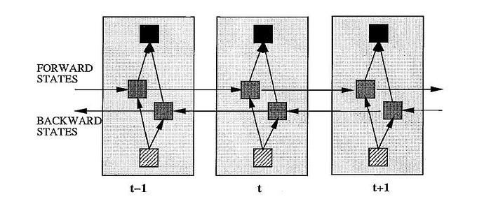
In training of BRNN, It can principally be trained with the same algorithms as a regular unidirectional RNN because there are no interactions between the two types of state neurons and, therefore, can be unfolded into a general feed-forward network. However, if, for example, any form of backpropagation through time (BPTT) is used, the forward and backward pass procedure is slightly more complicated because the update of state and output neurons can no longer be done one at a time.
The python code for BRNN is as below,
def BiRNN(x, weights, biases, timesteps, num_hidden):
    # Current data input shape: (batch_size, timesteps, n_input)

   # Unstack to get a list of 'timesteps' tensors of shape (batch_size, num_input)    x = tf.unstack(x, timesteps, 1)

    # Forward direction cell
    lstm_fw_cell = rnn.BasicLSTMCell(num_hidden, forget_bias=1.0)

    # Backward direction cell
    lstm_bw_cell = rnn.BasicLSTMCell(num_hidden, forget_bias=1.0)
    # Get BiRNN cell output
    outputs, _, _ = rnn.static_bidirectional_rnn(lstm_fw_cell, lstm_bw_cell, x,
                                                 dtype=tf.float32)
    # Linear activation, using rnn inner loop last output
    return tf.matmul(outputs[-1], weights) + biases
In the above code, we used a linear activation function. It is used at just one place i.e. output layer. No matter how many layers we have, if all are linear in nature, the final activation function of the last layer is nothing but just a linear function of the input of the first layer.
BiDirectional Attention Flow Model
Bi-Directional Attention Flow (BIDAF) network, a hierarchical multi-stage architecture for modeling the representations of the context paragraph at different levels of granularity. BIDAF includes character-level, word-level, and contextual embeddings. The bi-directional attention flow to obtain a query-aware context representation. Our attention mechanism offers the following improvements to the previously popular attention paradigms. First, our attention layer is not used to summarize the context paragraph into a fixed-size vector. Instead, the attention is computed for every time step, and the attended vector at each time step, along with the representations from previous layers, is allowed to flow through to the subsequent modeling layer.
The picture below shows that how BiDirectional Attention Flow Model works,

Here we can see that there are six hierarchical multistage process presents which are as below,
i. The Character Embedding Layer which maps each word to a vector space using character-level CNNs.
ii. The Word Embedding Layer maps each word to a vector space using a pre-trained word embedding model.
iii. The Contextual Embedding Layer utilizes contextual cues from surrounding words to refine the embedding of the words.
iv. Attention Flow Layer couples the query and context vectors and produces a set of query aware feature vectors for each word in the context.
v. Modeling Layer employs a Recurrent Neural Network to scan the context.
vi. Output Layer provides an answer to the query.
Here the first three layers applied to both query and context.
In the case of Bidirectional LSTM model with attention model, it utilizes neural attention mechanism with Bidirectional Long Short-Term Memory Networks(BLSTM) to capture the most important semantic information in a sentence. This model doesn’t utilize any features derived from lexical resources or NLP systems.

Hereby using BLSTM with attention mechanism, which can automatically focus on the words that have a decisive effect on classification, to capture the most important semantic information in a sentence. In the above mechanism, we have the following layers as,
i. Input layer: This layer is used for input the sentence to this model.
ii. Embedding layer: In this layer, it maps each word into a low dimension vector;
iii. LSTM layer: It utilizes BLSTM to get high-level features from the embedding layer.
iv. Attention layer: This layer produces a weight vector, and merge word-level features from each time step into a sentence-level feature vector, by multiplying the weight vector
v. Output layer: This layer is for the sentence-level feature vector which is finally used for relation classification.
The code for this model is available on https://github.com/kwonmha/Bidirectional-LSTM-with-attention-for-relation-classification/blob/master/att_bilstm.py
Multi-head Attention Mechanism
An attention function can be described as mapping a query and a set of key-value pairs to an output, where the query, keys, values, and output are all vectors. The output is computed as a weighted sum of the values, where the weight assigned to each value is computed by a compatibility function of the query with the corresponding key.
The context vector obtained by traditional attention mechanism focuses on a specific representation subspace of the input sequence. Such a context vector is expected to reflect one aspect of the semantics in the input. However, a sentence usually involves multiple semantics spaces, especially for a long sentence. In case of multi-head attention mechanism for Seq2Seq model to allow the decoder RNN to jointly attend to information from different representation subspaces of the encoder hidden states at the decoding process. The idea of multi-head has been applied to learn the sentence representation in self-attention.
The picture below is the simple architecture of encoder-decoder with multi-head attention,
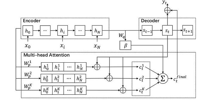
In “encoder-decoder attention” layers, the queries come from the previous decoder layer, and the memory keys and values come from the output of the encoder. This allows every position in the decoder to attend overall positions in the input sequence. The encoder contains self-attention layers. In a self-attention layer, all of the keys, values, and queries come from the same place, in this case, the output of the previous layer in the encoder. Each position in the encoder can attend to all positions in the previous layer of the encoder. Similarly, self-attention layers in the decoder allow each position in the decoder to attend to all positions in the decoder up to and including that position. We need to prevent leftward information flow in the decoder to preserve the auto-regressive property. We implement this inside of scaled dot-product attention by masking out (setting to −∞) all values in the input of the softmax which correspond to illegal connections.
The code for this model is available on
Sequence to Sequence Model with attention
Sequence-to-sequence model (Seq2Seq) was first proposed in machine translation. The idea was to translate one sequence to another sequence through an encoder-decoder neural architecture. Recently, dialog generation has been treated as sequence translation from a query to a reply. we use the attention based approach as it provides an effective methodology to perform sequence-to-sequence (seq2seq) training. We have encoder neural network which encodes the input sequence into a vector which has a fixed length and decoder neural network will generate each of words in the output sequence in turn, which is based on vector c and previously predicted words until it meets the word ending the sentence. In the seq2seq model, we can use different network architectures for encoder and decoder networks such as RNN or convolutional neural network.
The basic seq2seq model has the disadvantage of requiring the RNN decoder to use the entire encoding information from the input sequence whether the sequence is long or short. Secondly, the RNN encoder needs to encode the input sequence into a single vector which has a fixed length. This constraint is not really effective because, in fact, word generation at a time step in the output sequence sometimes depends more on certain components in the input sequence. For example, when translating a sentence from one language into another, we are more concerned about the context surrounding the current word compared to the other words in the sentence. The attention technique is given to solve that problem.
At the abstract level, attention loosens the condition that the entire input sequence is encoded by a single vector. Instead, the words in the input sequence will be encoded by the RNN encoder into a sequence of vectors. Then the RNN decoder applies soft attention technique by taking the weighted sum of the encoded vectors. The weighted sum of in this model is calculated by a feed-forward neural network. RNN encoder, RNN decoder, and parameters in attention are trained jointly from the data.
The picture below shows that working of encoder-decoder with attention,
A number of studies in machine translation combine the seq2seq model based on word embedding technique with the seq2seq model based on character embedding technique to improve the translation of out-of-vocabulary words. An important problem in the handling of historical texts is the normalization of words in historical texts on modern writing. In particular, the problem of normalization of historical texts is the main problem, and the auxiliary task is the mathematical model of grammatical-to-phoneme. Multi-task learning in the seq2seq model is accomplished by adding a classifier in the output layer of the network.
We can use the following code for this model,
https://github.com/farizrahman4u/seq2seq/blob/master/seq2seq/models.py
Character-based convolutional gated recurrent encoder with a word-based gated recurrent decoder with attention
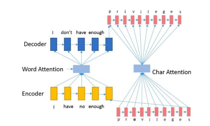
In this model, both the encoder and the decoder operate at the character level. Here sequence-to sequence character embedding in the encoder with word-based attention decoder, with openly accessible training data and the trained model for inference. This model has a similar underlying architecture of the sequence-to-sequence models used in machine translation. Sequence learning problems are challenging as deep neural networks (DNN) require the dimensionality of the inputs and targets to be fixed. Further, problems arise if the inputs are character concatenated representations whereas the outputs are word level representations. Therefore, in our model, the encoder is composed of both recurrent and feedforward units and operates at a character level whereas the decoder operates at a word level. Our model is composed on two main modules: Error Corrector Encoding Layer and Language Decoding Layer.
The illustrated picture is for a character-based convolutional gated recurrent encoder with the word-based gated recurrent decoder with attention,
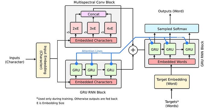
Here in Character Error Correcting Encoding Layer, we know that the Recurrent Neural Networks are extremely efficient in capturing contextual patterns. For a sequence of inputs, a classical RNN computes a sequence of outputs. The power of RNNs lies in the ease with which it can map input sequence to target sequence when the alignment between sequence is known ahead of time. In case of unaligned sequences, to circumvent the problem, the input and target sequences are padded to fixed length vectors, then one RNN is used as the encoder to map the padded input vector to a different fixed sized target vector using another RNN. However, RNNs struggle to cope with long term dependency in the data due to vanishing gradient problem. This problem is solved using Long Short Term Memory (LSTM) recurrent neural networks. However, for purposes of error correction, medium to short term dependencies are more useful. Therefore, our candidate for contextual error correction encoding layer is the Gated Recurrent Network (GRU) which has similar performance to that of LSTM.
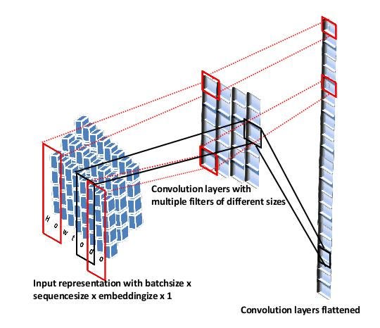
In Word Level Decoder the Implicit Language Model the decoder is also a GRU recurrent network that does word based processing. The output from the encoder is a linear transformation between the final hidden state of the char based GRU in the encoder and the output of the fully connected layer of the CNN. This state is then used to initialize the state of the decoder. The decoder sees as input a padded fixed length vector of integer indexes corresponding to the word in the vocabulary. The encoder-decoder is trained end-to-end having a combined char-word based representation on the encoder and decoder side respectively. The size of the GRU Word Level Decoder — Implicit Language Model The decoder is also a GRU recurrent network that does word based processing. The output from the encoder is a linear transformation between the final hidden state of the char based GRU in the encoder and the output of the fully connected layer of the CNN. This state is then used to initialize the state of the decoder. The decoder sees as input a padded fixed length vector of integer indexes corresponding to the word in the vocabulary. The input sequence is a sequence of words prefixed with the start token. The encoder-decoder is trained end-to-end having a combined char-word based representation on the encoder and decoder side respectively.
The picture below shows how CNN module comprising the encoder of CCEAD model used for capturing hidden representations,
We can use the code below for this model,
https://github.com/xiaodongdreams/attention-module/blob/master/MODELS/cbam.py
Conditional Sequence Generative Adversarial Nets
Generative adversarial network has enjoyed great success in computer vision and has been widely applied to image generation. The conditional generative adversarial nets apply an extension of the generative adversarial network to a conditional setting, which enables the networks to condition on some arbitrary external data. Some recent works have begun to apply the generative adversarial training into the NLP area: we can apply the idea of generative adversarial training to sentiment analysis and use the idea to domain adaptation tasks. For sequence generation problem, leverage policy gradient reinforcement learning to back-propagate the reward from the discriminator, showing presentable results for poem generation, speech-language generation and music generation.
In case of SeqGAN, It uses policy gradient to solve the intractable back- propagation issue, but a common problem in reinforcement learning appears sparse reward, that the non-zero reward is only observed at the last time step. The primary disadvantage of sparse reward is making the training sample inefficient. The inefficiency slows down training because the generator has a very little successful experience. Sparse reward causes another problem to chit-chat chatbot. In chatting, an incorrect response and a correct one can share the same prefix. For example, “I’m John.” and “I’m sorry.” have the same prefix “I’m”. But for the input “What ’s your name?”, the first response is reasonable and the second one is weak. The same prefix then receives the opposite feedback. The phenomenon continuously happens during training; the training signals become highly variant. The training is therefore unstable to deal with sparse reward, the original SeqGAN is trained with a stepwise evaluation method — Monte Carlo tree search (MCTS) . MCTS stabilizes the training, but it is computationally intractable when dealing with large dataset. To meet the necessity of large dataset for chatbot, a reward at every generation step (REGS) is proposed to replace MCTS but with worse performance. The motivation is to use a discriminator to estimate immediate rewards without computing a complex tree search. StepGAN only needs very little modification on discriminator and has significantly less computational costs than MCTS. We compare different GAN-based sequence generation approaches on a synthetic task and chit-chat dialogue generation. StepGAN outperforms MCTS and REGS on the synthetic task and generates more informative responses than other approaches in dialogue generation. Although we only apply StepGAN on dialogue generation. for example, machine translation, text summarization, and video caption generation.
The picture illustrated below shows that how generator and discriminator working in GAN,

With the help of Generative adversarial network, we can generate the text from random noise via adversarial training. In the case of GAN for dialogue generation, it uses a hierarchical long-short-term memory (LSTM) architecture for the discriminator. In contrast to their approach, we can apply the CNN-based discriminator for the machine translation task. Furthermore, we can also utilize the sentence-level bilingual evaluation understudy algo (BLEU) as the specific objective for the generator.
we can use the following code for SeqGAN Model,
https://github.com/LantaoYu/SeqGAN/blob/master/sequence_gan.py
Sequence to Sequence Encoding Decoding Architecture
Sequence-to-sequence learning (Seq2Seq) is about training models to convert sequences from one domain to sequences in another domain. When both input sequences and output sequences have the same length, you can implement such models simply with a Keras LSTM or GRU layer. see an example below,
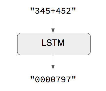
One caveat of this approach is that it assumes that it is possible to generate target given input. That works in some cases (e.g. adding strings of digits) but does not work for most use cases. In the general case, information about the entire input sequence is necessary in order to start generating the target sequence.
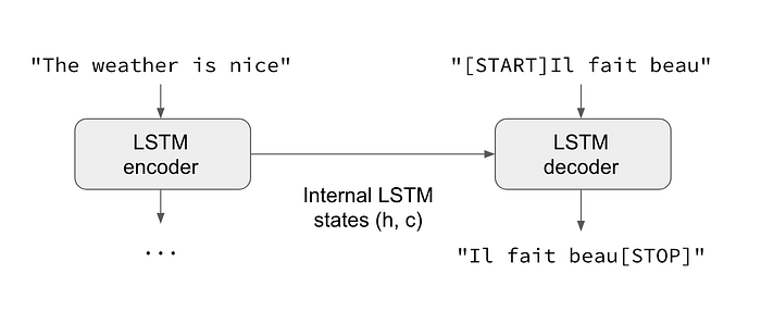
In the general case, input sequences and output sequences have different lengths (e.g. machine translation) and the entire input sequence is required in order to start predicting the target. This requires a more advanced setup, which is what people commonly refer to when mentioning “sequence to sequence models” with no further context. Here’s how it works:
- An RNN layer acts as “encoder”: it processes the input sequence and returns its own internal state.
- Another RNN layer (or stack thereof) acts as “decoder”: it is trained to predict the next characters of the target sequence, given previous characters of the target sequence. Specifically, it is trained to turn the target sequences into the same sequences but offset by one timestep in the future, a training process called “teacher forcing” in this context. Consider an example of language translation using a sequence to sequence model as
For applications, in general, if you can form your problem into an input sequence and an output sequence that you want to predict, seq2seq is likely a good approach. The basic setup is an encoder and a decoder, which consist of memory cells (LSTM/GRU) that help the network to remember long sequences. We can see the basic example as below,

We can use the following code for this model architecture,
https://github.com/atpaino/deep-text-corrector/blob/master/seq2seq.py
Bahdanau attention
In the regular seq2seq model, we embed our input sequence into a context vector, which is then used to make predictions. In the attention variant, the context vector is replaced by a customized context for the hidden decoder vector. The result is the sum over contribution over all of the input hidden vectors. Attention is important for the model to generalize well to test data, in that our model might learn to minimize the cost function during train time, but it is only when it learns attention that we know that it has an idea that it knows exactly where to look (and put that knowledge into the context) for it to generalize well to test data.
In Bahdanau attention model use the concatenation of the forward and backward source hidden states in the bi-directional encoder and target hidden states in their non-stacking unidirectional decoder. Bahdanau has only concat score alignment model.

The picture illustrated below shows how the attention mechanism works

We can use the following code for this model,
LSTM Neural Networks for Language Modeling
Language modeling is the art of determining the probability of a sequence of words. This is useful in a large variety of areas including speech recognition, optical character recognition, handwriting recognition, machine translation, and spelling correction.
The goal of statistical language modeling is to predict the next word in textual data given context; thus we are dealing with sequential data prediction problem when constructing language models. Still, many attempts to obtain such statistical models involve approaches that are very specific for language domain — for example, assumption that natural language sentences can be described by parse trees, or that we need to consider morphology of words, syntax, and semantics. Even the most widely used and general models, based on n-gram statistics, assume that language consists of sequences of atomic symbols — words — that form sentences, and where the end of sentence symbol plays important and very special role. Language models for real-world speech recognition or machine translation systems are built on huge amounts of data, and popular belief says that more data is all we need. Neural language models take advantage of word order, and state the same assumption as n-gram models that words closer in a sequence are statistically more dependent. Typically, a neural language model learns the probability distribution of the next word given a fixed number of preceding words which act as the context.
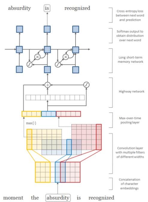
The illustrated picture has three types (a) is a standard LSTM LM. (b) represents an LM where both input and Softmax embeddings have been replaced by a character CNN. (c) Next character prediction LSTM network.

Neural network LMs always estimate probabilities based on the full history, regardless of whether the n-gram was seen in training or not. On the other hand, the n-gram assumption still leads to an inaccuracy in the modeling when feed-forward neural network LMs are used. Unfortunately, recurrent neural networks are hard to train using backpropagation through time. The main difficulty lies in the well-known vanishing gradient problem which means that the gradient that is propagated back through the network either decays or grows exponentially. One approach to improved training of recurrent neural networks lies in better optimization algorithms that make use of higher-order information. However, this usually comes at the price of significantly increased computational costs which makes these methods less attractive for language modeling where the amount of training data is extremely large. An alternative solution called Long Short-Term Memory (LSTM) in which network architecture is modified such that the vanishing gradient problem is explicitly avoided, whereas the training algorithm is left unchanged.
The picture below shows how the language model works,
We can use the following code for language modeling,
https://github.com/SudaMonster/lstm-language-model/blob/master/model.py
3. Coding and Model Architecture for the spelling correction
In this spelling correction project, I will use Bi-directional RNN in the encoding layer and Bahdanau Attention in the decoding layer. I will also use a grid search to find the optimal architecture and hyperparameter value. For this, I will use the dataset having twenty popular books from [Project Gutenberg (http://www.gutenberg.org/ebooks/search/?sort_order=downloads).
There are following steps which I will follow,
- Loading the Data
- Preparing the Data
- Building the Model
- Training the Model
- Fixing Custom Sentences
- Summary
The code is available on my Github profile,
https://github.com/kunalBhashkar/tensorflow_spelling_correction
4. Results and Conclusion
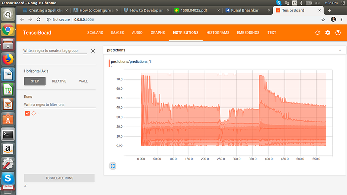
We have presented a new error model for noisy channel spelling correction based on a generic string to string edits, and have demonstrated that it results in a significant improvement in performance compared to previous approaches. The best results, as measured by sequence loss with 15% of our data. We can see the model structure, prediction, and cost function on the tensorboard.
Output:
We got some text and their response as below,
text = "The first days of her existence in th country were vrey hard for Dolly.."Response:
Response Words: The first days of her existence in th country were vere vre hard for Dolly.Another example,text = "Thi is really something impressiv thaat we should look into right away!"Response Words: Thi is really something impressive that we should look into right away! i
To run TensorBoard, we can use the following command,
tensorboard --logdir=path/to/log-directory


5. References
i. ABCNN: Attention-Based Convolutional Neural Network for Modeling Sentence Pairs (paper)
ii. An Unsupervised and Data-Driven Approach for Spell Checking in
Vietnamese OCR-scanned Texts (paper)
iii. NEURAL MACHINE TRANSLATION BY JOINTLY LEARNING TO ALIGN AND TRANSLATE(paper)
iv. Effective Approaches to Attention-based Neural Machine Translation(paper)
v. Google’s Neural Machine Translation System: Bridging the Gap
between Human and Machine Translation(paper)
vi. B I -DIRECTIONAL ATTENTION FLOW FOR MACHINE COMPREHENSION(paper)
vii. Towards better decoding and language model integration in sequence to
sequence models(paper)
viii. Character-based Joint Segmentation and POS Tagging for Chinese
using Bidirectional RNN-CRF (paper)
ix. Attention Is All You Need (paper)
x. Coherent Dialogue with Attention-Based Language Models(paper)
xi. HYBRID SPEECH RECOGNITION WITH DEEP BIDIRECTIONAL LSTM(paper)
xii. Bidirectional Recurrent Neural Networks (paper)
xiii. Named Entity Recognition with Bidirectional LSTM-CNNs (paper)
xiv. Bidirectional Recurrent Neural Networks (paper)
xv. A Neural Probabilistic Language Model (paper)
